OpenCV 图像处理：几何变换、图像缩放、图像平移、图像旋转、仿射变换、透射变换、图像金字塔

日萌社

人工智能AI：Keras PyTorch MXNet TensorFlow PaddlePaddle 深度学习实战（不定时更新）

---

几何变换

学习目标

• 掌握图像的缩放，平移，旋转等
• 了解数字图像的仿射变换和透射变换

---

1 图像缩放

缩放是对图像的大小进行调整，即使图像放大或缩小。

1. API

   cv2.resize(src,dsize,fx=0,fy=0,interpolation=cv2.INTER_LINEAR)
   

   参数：

   • src : 输入图像

   • dsize: 绝对尺寸，直接指定调整后图像的大小

   • fx,fy: 相对尺寸，将dsize设置为None，然后将fx和fy设置为比例因子即可

   • interpolation：插值方法，

1. 示例

2. import cv2 as cv
   # 1. 读取图片
   img1 = cv.imread("./image/dog.jpeg")
   # 2.图像缩放
   # 2.1 绝对尺寸
   rows,cols = img1.shape[:2]
   res = cv.resize(img1,(2*cols,2*rows),interpolation=cv.INTER_CUBIC)
   
   # 2.2 相对尺寸
   res1 = cv.resize(img1,None,fx=0.5,fy=0.5)
   
   # 3 图像显示
   # 3.1 使用opencv显示图像(不推荐)
   cv.imshow("orignal",img1)
   cv.imshow("enlarge",res)
   cv.imshow("shrink）",res1)
   cv.waitKey(0)
   
   # 3.2 使用matplotlib显示图像
   fig,axes=plt.subplots(nrows=1,ncols=3,figsize=(10,8),dpi=100)
   axes[0].imshow(res[:,:,::-1])
   axes[0].set_title("绝对尺度（放大）")
   axes[1].imshow(img1[:,:,::-1])
   axes[1].set_title("原图")
   axes[2].imshow(res1[:,:,::-1])
   axes[2].set_title("相对尺度（缩小）")
   plt.show()

2 图像平移

图像平移将图像按照指定方向和距离，移动到相应的位置。

1. API

cv.warpAffine(img,M,dsize)

参数：

• img: 输入图像

• M： 2*∗3移动矩阵

• 注意：将M设置为np.float32类型的Numpy数组。

• dsize: 输出图像的大小

  注意：输出图像的大小，它应该是(宽度，高度)的形式。请记住,width=列数，height=行数。

• 示例

需求是将图像的像素点移动(50,100)的距离：

import numpy as np
import cv2 as cv
import matplotlib.pyplot as plt
# 1. 读取图像
img1 = cv.imread("./image/image2.jpg")

# 2. 图像平移
rows,cols = img1.shape[:2]
M = M = np.float32([[1,0,100],[0,1,50]])# 平移矩阵
dst = cv.warpAffine(img1,M,(cols,rows))

# 3. 图像显示
fig,axes=plt.subplots(nrows=1,ncols=2,figsize=(10,8),dpi=100)
axes[0].imshow(img1[:,:,::-1])
axes[0].set_title("原图")
axes[1].imshow(dst[:,:,::-1])
axes[1].set_title("平移后结果")
plt.show()

3 图像旋转

图像旋转是指图像按照某个位置转动一定角度的过程，旋转中图像仍保持这原始尺寸。图像旋转后图像的水平对称轴、垂直对称轴及中心坐标原点都可能会发生变换，因此需要对图像旋转中的坐标进行相应转换。

那图像是怎么进行旋转的呢？如下图所示：

同时我们要修正原点的位置，因为原图像中的坐标原点在图像的左上角，经过旋转后图像的大小会有所变化，原点也需要修正。

假设在旋转的时候是以旋转中心为坐标原点的，旋转结束后还需要将坐标原点移到图像左上角，也就是还要进行一次变换。

在OpenCV中图像旋转首先根据旋转角度和旋转中心获取旋转矩阵，然后根据旋转矩阵进行变换，即可实现任意角度和任意中心的旋转效果。

1. API

   cv2.getRotationMatrix2D(center, angle, scale)
   

   参数：

   • center：旋转中心
   • angle：旋转角度
   • scale：缩放比例

   返回：

   • M：旋转矩阵

     调用cv.warpAffine完成图像的旋转

2. 示例

   import numpy as np
   import cv2 as cv
   import matplotlib.pyplot as plt
   # 1 读取图像
   img = cv.imread("./image/image2.jpg")
   
   # 2 图像旋转
   rows,cols = img.shape[:2]
   # 2.1 生成旋转矩阵
   M = cv.getRotationMatrix2D((cols/2,rows/2),90,1)
   # 2.2 进行旋转变换
   dst = cv.warpAffine(img,M,(cols,rows))
   
   # 3 图像展示
   fig,axes=plt.subplots(nrows=1,ncols=2,figsize=(10,8),dpi=100)
   axes[0].imshow(img1[:,:,::-1])
   axes[0].set_title("原图")
   axes[1].imshow(dst[:,:,::-1])
   axes[1].set_title("旋转后结果")
   plt.show()

4 仿射变换

图像的仿射变换涉及到图像的形状位置角度的变化，是深度学习预处理中常到的功能,仿射变换主要是对图像的缩放，旋转，翻转和平移等操作的组合。

那什么是图像的仿射变换，如下图所示，图1中的点1, 2 和 3 与图二中三个点一一映射, 仍然形成三角形, 但形状已经大大改变，通过这样两组三点（感兴趣点）求出仿射变换， 接下来我们就能把仿射变换应用到图像中所有的点中，就完成了图像的仿射变换。

需要注意的是，对于图像而言，宽度方向是x，高度方向是y，坐标的顺序和图像像素对应下标一致。所以原点的位置不是左下角而是右上角，y的方向也不是向上，而是向下。

在仿射变换中，原图中所有的平行线在结果图像中同样平行。为了创建这个矩阵我们需要从原图像中找到三个点以及他们在输出图像中的位置。然后cv2.getAffineTransform 会创建一个 2x3 的矩阵，最后这个矩阵会被传给函数 cv2.warpAffine。

示例

import numpy as np
import cv2 as cv
import matplotlib.pyplot as plt
# 1 图像读取
img = cv.imread("./image/image2.jpg")

# 2 仿射变换
rows,cols = img.shape[:2]
# 2.1 创建变换矩阵
pts1 = np.float32([[50,50],[200,50],[50,200]])
pts2 = np.float32([[100,100],[200,50],[100,250]])
M = cv.getAffineTransform(pts1,pts2)
# 2.2 完成仿射变换
dst = cv.warpAffine(img,M,(cols,rows))

# 3 图像显示
fig,axes=plt.subplots(nrows=1,ncols=2,figsize=(10,8),dpi=100)
axes[0].imshow(img[:,:,::-1])
axes[0].set_title("原图")
axes[1].imshow(dst[:,:,::-1])
axes[1].set_title("仿射后结果")
plt.show()

5 透射变换

透射变换是视角变化的结果，是指利用透视中心、像点、目标点三点共线的条件，按透视旋转定律使承影面（透视面）绕迹线（透视轴）旋转某一角度，破坏原有的投影光线束，仍能保持承影面上投影几何图形不变的变换。

示例

import numpy as np
import cv2 as cv
import matplotlib.pyplot as plt
# 1 读取图像
img = cv.imread("./image/image2.jpg")
# 2 透射变换
rows,cols = img.shape[:2]
# 2.1 创建变换矩阵
pts1 = np.float32([[56,65],[368,52],[28,387],[389,390]])
pts2 = np.float32([[100,145],[300,100],[80,290],[310,300]])

T = cv.getPerspectiveTransform(pts1,pts2)
# 2.2 进行变换
dst = cv.warpPerspective(img,T,(cols,rows))

# 3 图像显示
fig,axes=plt.subplots(nrows=1,ncols=2,figsize=(10,8),dpi=100)
axes[0].imshow(img[:,:,::-1])
axes[0].set_title("原图")
axes[1].imshow(dst[:,:,::-1])
axes[1].set_title("透射后结果")
plt.show()

6 图像金字塔

图像金字塔是图像多尺度表达的一种，最主要用于图像的分割，是一种以多分辨率来解释图像的有效但概念简单的结构。

图像金字塔用于机器视觉和图像压缩，一幅图像的金字塔是一系列以金字塔形状排列的分辨率逐步降低，且来源于同一张原始图的图像集合。其通过梯次向下采样获得，直到达到某个终止条件才停止采样。

金字塔的底部是待处理图像的高分辨率表示，而顶部是低分辨率的近似，层级越高，图像越小，分辨率越低。

1. API

   cv.pyrUp(img)       #对图像进行上采样
   cv.pyrDown(img)        #对图像进行下采样
   

2. 示例

   import numpy as np
   import cv2 as cv
   import matplotlib.pyplot as plt
   # 1 图像读取
   img = cv.imread("./image/image2.jpg")
   # 2 进行图像采样
   up_img = cv.pyrUp(img)  # 上采样操作
   img_1 = cv.pyrDown(img)  # 下采样操作
   # 3 图像显示
   cv.imshow('enlarge', up_img)
   cv.imshow('original', img)
   cv.imshow('shrink', img_1)
   cv.waitKey(0)
   cv.destroyAllWindows()
   

总结

1. 图像缩放：对图像进行放大或缩小

   cv.resize()

2. 图像平移：

   指定平移矩阵后，调用cv.warpAffine()平移图像

3. 图像旋转：

   调用cv.getRotationMatrix2D获取旋转矩阵，然后调用cv.warpAffine()进行旋转

4. 仿射变换：

   调用cv.getAffineTransform将创建变换矩阵，最后该矩阵将传递给cv.warpAffine()进行变换

5. 透射变换：

   通过函数cv.getPerspectiveTransform()找到变换矩阵，将cv.warpPerspective()进行投射变换

6. 金字塔

   图像金字塔是图像多尺度表达的一种，使用的API：

   cv.pyrUp(): 向上采样

   cv.pyrDown(): 向下采样

---

双线性插值

双线性插值
	1.转置卷积层可以放大特征图。
	2.在图像处理中，我们有时需要将图像放大，即上采样（upsample）。
	 上采样的方法有很多，常用的有双线性插值。简单来说，为了得到输出图像在坐标(x, y)上的像素，
	 先将该坐标映射到输入图像的坐标(x′, y′)，例如，根据输入与输出的尺寸之比来映射。
	 映射后的x′和y′通常是实数。然后，在输入图像上找到与坐标(x′, y′)最近的4个像素。
	 最后，输出图像在坐标(x, y)上的像素依据输入图像上这4个像素及其与(x′, y′)的相对距离来计算。
	 双线性插值的上采样可以通过由以下bilinear_kernel函数构造的卷积核的转置卷积层来实现。
	3.数学里factor是因数的意思。2和3是6的因数。
	  假如a*b=c（a、b、c都是整数)，那么我们称a和b就是c的因数。 
	  需要注意的是，唯有被除数，除数，商皆为整数，余数为零时，此关系才成立。 
	  反过来说，我们称c为a、b的倍数。在研究因数和倍数时，不考虑0。


# 构造一个将输入的高和宽放大2倍的转置卷积层：设置步长strides=2
# Conv2DTranspose转置卷积层:输出通道数为3，卷积核大小4x4，填充1，步长2
conv_trans = nn.Conv2DTranspose(3, kernel_size=4, padding=1, strides=2)
# bilinear_kernel()函数返回初始化好的kernel卷积核
conv_trans.initialize(init.Constant(bilinear_kernel(3, 3, 4)))
 
def bilinear_kernel(in_channels, out_channels, kernel_size):
	# 因数2 = (4 + 1) // 2
	factor = (kernel_size + 1) // 2
	# 奇数%2==1，偶数%2==0。4%2==0
	if kernel_size % 2 == 1:
		center = factor - 1
	else:
		# center = 1.5 = 2- 0.5
		center = factor - 0.5
	# og[0].shape = (4, 1) 。og[1].shape = (1, 4)
	og = np.ogrid[:kernel_size, :kernel_size]
	# filt.shape = (4, 4)
	filt = (1 - abs(og[0] - center) / factor) * (1 - abs(og[1] - center) / factor)
	# weight.shape = (3, 3, 4, 4)
	weight = np.zeros((in_channels, out_channels, kernel_size, kernel_size), dtype='float32')
	weight[range(in_channels), range(out_channels), :, :] = filt
	# 返回的数组shape为(3, 3, 4, 4)
	return nd.array(weight)

下面为og、filt、weight的打印值情况：
		og = [array([[0],
			    [1],
			    [2],
			    [3]]), 
		       array([[0, 1, 2, 3]])]
			
		filt = array([[0.0625, 0.1875, 0.1875, 0.0625],
			     [0.1875, 0.5625, 0.5625, 0.1875],
			     [0.1875, 0.5625, 0.5625, 0.1875],
			     [0.0625, 0.1875, 0.1875, 0.0625]])
		 
		weight = array([[[[0.0625, 0.1875, 0.1875, 0.0625],
				[0.1875, 0.5625, 0.5625, 0.1875],
				[0.1875, 0.5625, 0.5625, 0.1875],
				[0.0625, 0.1875, 0.1875, 0.0625]],
				[[0.    , 0.    , 0.    , 0.    ],
				[0.    , 0.    , 0.    , 0.    ],
				[0.    , 0.    , 0.    , 0.    ],
				[0.    , 0.    , 0.    , 0.    ]],
				[[0.    , 0.    , 0.    , 0.    ],
				[0.    , 0.    , 0.    , 0.    ],
				[0.    , 0.    , 0.    , 0.    ],
				[0.    , 0.    , 0.    , 0.    ]]],
			
				[[[0.    , 0.    , 0.    , 0.    ],
				[0.    , 0.    , 0.    , 0.    ],
				[0.    , 0.    , 0.    , 0.    ],
				[0.    , 0.    , 0.    , 0.    ]],
				[[0.0625, 0.1875, 0.1875, 0.0625],
				[0.1875, 0.5625, 0.5625, 0.1875],
				[0.1875, 0.5625, 0.5625, 0.1875],
				[0.0625, 0.1875, 0.1875, 0.0625]],
				[[0.    , 0.    , 0.    , 0.    ],
				[0.    , 0.    , 0.    , 0.    ],
				[0.    , 0.    , 0.    , 0.    ],
				[0.    , 0.    , 0.    , 0.    ]]],
				
				[[[0.    , 0.    , 0.    , 0.    ],
				[0.    , 0.    , 0.    , 0.    ],
				[0.    , 0.    , 0.    , 0.    ],
				[0.    , 0.    , 0.    , 0.    ]],
				[[0.    , 0.    , 0.    , 0.    ],
				[0.    , 0.    , 0.    , 0.    ],
				[0.    , 0.    , 0.    , 0.    ],
				[0.    , 0.    , 0.    , 0.    ]],
				[[0.0625, 0.1875, 0.1875, 0.0625],
				[0.1875, 0.5625, 0.5625, 0.1875],
				[0.1875, 0.5625, 0.5625, 0.1875],
				[0.0625, 0.1875, 0.1875, 0.0625]]]], dtype=float32) 
		 

						   
# 读取图像X，将上采样的结果记作Y。为了打印图像，我们需要调整通道维的位置。	
img = image.imread('../img/catdog.jpg') 
# transpose((2, 0, 1)) 表示把读取图像X的 高x宽x通道数 变换为 通道数x高x宽
X = img.astype('float32').transpose((2, 0, 1)).expand_dims(axis=0) / 255
Y = conv_trans(X)
# 上采样的结果记作Y。transpose((1, 2, 0))表示把上采样的结果的 通道数x高x宽 变换为 高x宽x通道数
out_img = Y[0].transpose((1, 2, 0))

# 可以看到，转置卷积层将图像的高和宽分别放大2倍。值得一提的是，除了坐标刻度不同，
# 双线性插值放大的图像和“目标检测和边界框”一节中打印出的原图看上去没什么两样。
d2l.set_figsize()
print('input image shape:', img.shape)
d2l.plt.imshow(img.asnumpy());
print('output image shape:', out_img.shape)
d2l.plt.imshow(out_img.asnumpy());

input image shape: (561, 728, 3)
output image shape: (1122, 1456, 3)

---

In [1]:

import numpy as np

import cv2 as cv

import matplotlib.pyplot as plt

In [2]:

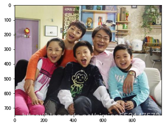
kids = cv.imread("./image/kids.jpg")

In [3]:

plt.imshow(kids[:,:,::-1])

Out[3]:

<matplotlib.image.AxesImage at 0x120089ed0>

图像缩放

In [4]:

# 绝对尺寸

rows,cols = kids.shape[:2]

In [5]:

rows

Out[5]:

374

In [6]:

cols

Out[6]:

500

In [7]:

res = cv.resize(kids,(2*cols,2*rows))

In [8]:

plt.imshow(res[:,:,::-1])

Out[8]:

<matplotlib.image.AxesImage at 0x12068c510>

In [9]:

res.shape

Out[9]:

(748, 1000, 3)

In [10]:

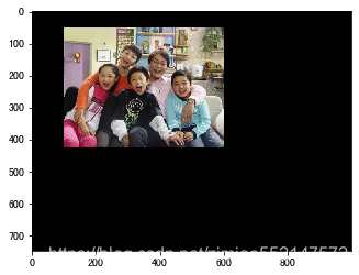
res1 = cv.resize(kids,None,fx=0.5,fy=0.5)

In [11]:

plt.imshow(res1[:,:,::-1])

Out[11]:

<matplotlib.image.AxesImage at 0x1207045d0>

In [12]:

res1.shape

Out[12]:

(187, 250, 3)

图像平移

In [13]:

plt.imshow(kids[:,:,::-1])

Out[13]:

<matplotlib.image.AxesImage at 0x127b901d0>

In [14]:

rows

Out[14]:

374

In [15]:

cols

Out[15]:

500

In [16]:

M = np.float32([[1,0,100],[0,1,50]])

In [19]:

res2 = cv.warpAffine(kids,M,(2*cols,2*rows))

In [20]:

plt.imshow(res2[:,:,::-1])

Out[20]:

<matplotlib.image.AxesImage at 0x1200e1d90>

图像旋转

In [35]:

M = cv.getRotationMatrix2D((cols/2,rows/2),45,0.5)

In [36]:

res3 = cv.warpAffine(kids,M,(cols,rows))

In [37]:

plt.imshow(res3[:,:,::-1])

Out[37]:

<matplotlib.image.AxesImage at 0x12b8d99d0>

仿射变换

In [41]:

pts1 = np.float32([[50,50],[200,50],[50,200]])

pts2 = np.float32([[100,100],[200,50],[100,250]])

In [42]:

M = cv.getAffineTransform(pts1,pts2)

In [43]:

M

Out[43]:

array([[ 0.66666667,  0.        , 66.66666667],
       [-0.33333333,  1.        , 66.66666667]])

In [44]:

res4 = cv.warpAffine(kids,M,(cols,rows))

In [45]:

plt.imshow(res4[:,:,::-1])

Out[45]:

<matplotlib.image.AxesImage at 0x12a928f10>

投射变换

In [59]:

pst1 = np.float32([[56,65],[368,52],[28,387],[389,390]])

pst2 = np.float32([[100,145],[300,100],[80,290],[310,300]])

In [61]:

T = cv.getPerspectiveTransform(pst1,pst2)

In [62]:

T

Out[62]:

array([[ 3.98327670e-01, -2.09876559e-02,  7.49460064e+01],
       [-1.92233080e-01,  4.29335771e-01,  1.21896057e+02],
       [-7.18774228e-04, -1.33393850e-05,  1.00000000e+00]])

In [63]:

res5 = cv.warpPerspective(kids,T,(cols,rows))

In [64]:

plt.imshow(res5[:,:,::-1])

Out[64]:

<matplotlib.image.AxesImage at 0x12d6d4410>

图像金字塔

In [65]:

plt.imshow(kids[:,:,::-1])

Out[65]:

<matplotlib.image.AxesImage at 0x12d44b890>

In [66]:

imgup = cv.pyrUp(kids)

In [67]:

plt.imshow(imgup[:,:,::-1])

Out[67]:

<matplotlib.image.AxesImage at 0x12ce20e50>

In [68]:

imgup2 = cv.pyrUp(imgup)

In [69]:

plt.imshow(imgup2[:,:,::-1])

Out[69]:

<matplotlib.image.AxesImage at 0x12d061c10>

In [71]:

imgdown = cv.pyrDown(kids)

In [73]:

plt.imshow(imgdown[:,:,::-1])

Out[73]:

<matplotlib.image.AxesImage at 0x12a3dc950>