[高光谱]PyTorch使用CNN对高光谱图像进行分类

项目原地址：

Hyperspectral-Classificationhttps://github.com/eecn/Hyperspectral-ClassificationDataLoader讲解：

[高光谱]使用PyTorch的dataloader加载高光谱数据https://blog.csdn.net/weixin_37878740/article/details/130929358

一、模型加载

        在原始项目中，提供了14种模型可供选择，从最简单的SVM到3D-CNN，这里以2D-CNN为例，在原项目中需要将model属性设置为：sharma。

         模型通过一个get_model(.)函数获得，该函数一共四个返回（model, optimizer, loss, hyperparams；分别为：模型，迭代器，损失函数，超参数），输入为模型类别。

        进入函数内部，找到对应的函数体如下：

elif name == 'sharma':
        kwargs.setdefault('batch_size', 60)        #batch_szie
        epoch = kwargs.setdefault('epoch', 30)     #迭代数
        lr = kwargs.setdefault('lr', 0.05)         #学习率
        center_pixel = True                        #是否开启中心像素模型
        # We assume patch_size = 64
        kwargs.setdefault('patch_size', 64)        #patch_szie，即图像块大小
        model = SharmaEtAl(n_bands, n_classes, patch_size=kwargs['patch_size'])  #模型本体
        optimizer = optim.SGD(model.parameters(), lr=lr, weight_decay=0.0005)    #迭代器
        criterion = nn.CrossEntropyLoss(weight=kwargs['weights'])            #交叉熵损失函数
        kwargs.setdefault('scheduler', optim.lr_scheduler.MultiStepLR(optimizer, milestones=[epoch // 2, (5 * epoch) // 6], gamma=0.1))

        这里设置了一部分超参数，同时设置了patch_size为64（此概念可以参见dataloader篇），采用的损失函数为常见的交叉熵损失函数，而模型本体则是使用SharmaEtAl(.)进行加载。

二、模型本体

        跳转至SharmaEtAl(nn.Module)，其继承自nn.model，输入参数3个，分别为：输入通道数、分类数、图块尺寸。

def __init__(self, input_channels, n_classes, patch_size=64):

  该网络的结构如图，模型中里面包含3个卷积、2个bn、2个池化和2个全连接，如下：

扫描二维码关注公众号，回复： 16949766 查看本文章

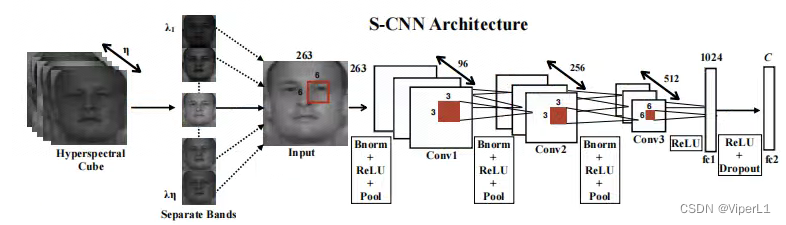
# 卷积层1
self.conv1 = nn.Conv3d(1, 96, (input_channels, 6, 6), stride=(1,2,2))
self.conv1_bn = nn.BatchNorm3d(96)
self.pool1 = nn.MaxPool3d((1, 2, 2))
# 卷积层2
self.conv2 = nn.Conv3d(1, 256, (96, 3, 3), stride=(1,2,2))
self.conv2_bn = nn.BatchNorm3d(256)
self.pool2 = nn.MaxPool3d((1, 2, 2))
# 卷积层3
self.conv3 = nn.Conv3d(1, 512, (256, 3, 3), stride=(1,1,1))

# 展平函数
self.features_size = self._get_final_flattened_size()

# 由两个全连接组成的分类器
self.fc1 = nn.Linear(self.features_size, 1024)
self.dropout = nn.Dropout(p=0.5)
self.fc2 = nn.Linear(1024, n_classes)

        其中的展平函数_get_final_flattened_size(.)，并不实际参与前向传递，仅计算转换后的通道数。

    def _get_final_flattened_size(self):
        with torch.no_grad():
            x = torch.zeros((1, 1, self.input_channels,
                             self.patch_size, self.patch_size))
            x = F.relu(self.conv1_bn(self.conv1(x)))
            x = self.pool1(x)
            print(x.size())
            b, t, c, w, h = x.size()
            x = x.view(b, 1, t*c, w, h) 
            x = F.relu(self.conv2_bn(self.conv2(x)))
            x = self.pool2(x)
            print(x.size())
            b, t, c, w, h = x.size()
            x = x.view(b, 1, t*c, w, h) 
            x = F.relu(self.conv3(x))
            print(x.size())
            _, t, c, w, h = x.size()
        return t * c * w * h

        实际的前向传递如下：

    def forward(self, x):
        # 卷积块1
        x = F.relu(self.conv1_bn(self.conv1(x)))
        x = self.pool1(x)
        # 获取tensor尺寸
        b, t, c, w, h = x.size()
        # 调整tensor尺寸
        x = x.view(b, 1, t*c, w, h) 
        # 卷积块2
        x = F.relu(self.conv2_bn(self.conv2(x)))
        x = self.pool2(x)
        # 获取tensor尺寸
        b, t, c, w, h = x.size()
        # 调整tensor尺寸
        x = x.view(b, 1, t*c, w, h) 
        # 卷积块3
        x = F.relu(self.conv3(x))
        # 调整tensor尺寸
        x = x.view(-1, self.features_size)
        # 分类器
        x = self.fc1(x)
        x = self.dropout(x)
        x = self.fc2(x)
        return x

三、训练与测试

        主函数中，训练和测试结构如下：

        try:
            train(model, optimizer, loss, train_loader, hyperparams['epoch'],
                  scheduler=hyperparams['scheduler'], device=hyperparams['device'],
                  supervision=hyperparams['supervision'], val_loader=val_loader,
                  display=viz)
        except KeyboardInterrupt:
            # Allow the user to stop the training
            pass

        probabilities = test(model, img, hyperparams)
        prediction = np.argmax(probabilities, axis=-1)

        训练被封装在train(.)函数中，测试封装在test(.)函数中，下面逐一来看。

        首先是train函数，这里省去外围部分，仅看核心的循环控制段。

# 外循环控制，用于控制轮次(epoch)
for e in tqdm(range(1, epoch + 1), desc="Training the network"):
        # 进入训练模式
        net.train()
        avg_loss = 0.

        # 从dataloader中取出图像(data)和标签(target)
        for batch_idx, (data, target) in tqdm(enumerate(data_loader), total=len(data_loader)):
            # 如果是GPU模式则需要转换为cuda格式
            data, target = data.to(device), target.to(device)

        #---实际的训练部分---#
            # 冻结梯度
            optimizer.zero_grad()
            # 训练模式（监督训练/半监督训练）
            if supervision == 'full':
                # 前向传递
                output = net(data)
                #target = target - 1
                # 交叉熵损失函数
                loss = criterion(output, target)
            elif supervision == 'semi':
                outs = net(data)
                output, rec = outs
                #target = target - 1
                loss = criterion[0](output, target) + net.aux_loss_weight * criterion[1](rec, data)
        #---实际的训练部分---#
            # 损失函数反向传递
            loss.backward()
            # 迭代器步进
            optimizer.step()

            # 记录损失函数
            avg_loss += loss.item()
            losses[iter_] = loss.item()
            mean_losses[iter_] = np.mean(losses[max(0, iter_ - 100):iter_ + 1])

            iter_ += 1
            del(data, target, loss, output)

        接下来是test函数，与train不同的是，其参数为：model, img, hyperparams。其中img，是一整张高光谱图像，而不是由DataSet块采样后的图像块。故其结构也与train大不相同。

        在进行测试的时候，需要一个滑动窗口(sliding_window)函数将其进行切块以满足图像输入的要求。同时还需要一个grouper函数将其组装为batch送入神经网络中。所以我们可以看到循环控制的最外层实际上就是上面两个函数来组成的。

    # 图像切块
    iterations = count_sliding_window(img, **kwargs) // batch_size
    for batch in tqdm(grouper(batch_size, sliding_window(img, **kwargs)),
                      total=(iterations),
                      desc="Inference on the image"
                      ):
        #  锁定梯度
        with torch.no_grad():
            #  逐像素模式
            if patch_size == 1:
                data = [b[0][0, 0] for b in batch]
                data = np.copy(data)
                data = torch.from_numpy(data)
            # 其他模式
            else:
                data = [b[0] for b in batch]
                data = np.copy(data)
                data = data.transpose(0, 3, 1, 2)
                data = torch.from_numpy(data)
                data = data.unsqueeze(1)

            indices = [b[1:] for b in batch]
            # 类型转换
            data = data.to(device)
            # 前向传递
            output = net(data)
            if isinstance(output, tuple):
                output = output[0]
            output = output.to('cpu')

            if patch_size == 1 or center_pixel:
                output = output.numpy()
            else:
                output = np.transpose(output.numpy(), (0, 2, 3, 1))
            for (x, y, w, h), out in zip(indices, output):

            # 将得到的像素平装回原尺寸
                if center_pixel:
                    probs[x + w // 2, y + h // 2] += out
                else:
                    probs[x:x + w, y:y + h] += out
    return probs

        这个函数会使用上述的两个函数，将图像切割成可以放入神经网络的尺寸并逐个进行前向传递，最后将得到的所有像素的结果按照原来的尺寸组成一个结果矩阵返回。

        最后，这个结果由一个argmax函数得到其概率最大的预测结果：

prediction = np.argmax(probabilities, axis=-1)

四、结果计算

        在完成上述步骤后，由metrics(.)函数计算最终的模型结果：

run_results = metrics(prediction, test_gt, ignored_labels=hyperparams['ignored_labels'], n_classes=N_CLASSES)

        其函数体如下：

def metrics(prediction, target, ignored_labels=[], n_classes=None):
    """Compute and print metrics (accuracy, confusion matrix and F1 scores).

    Args:
        prediction: list of predicted labels
        target: list of target labels
        ignored_labels (optional): list of labels to ignore, e.g. 0 for undef
        n_classes (optional): number of classes, max(target) by default
    Returns:
        accuracy, F1 score by class, confusion matrix
    """
    ignored_mask = np.zeros(target.shape[:2], dtype=np.bool)
    for l in ignored_labels:
        ignored_mask[target == l] = True
    ignored_mask = ~ignored_mask
    #target = target[ignored_mask] -1
    target = target[ignored_mask]
    prediction = prediction[ignored_mask]

    results = {}

    n_classes = np.max(target) + 1 if n_classes is None else n_classes

    cm = confusion_matrix(
        target,
        prediction,
        labels=range(n_classes))

    results["Confusion matrix"] = cm

    # Compute global accuracy
    total = np.sum(cm)
    accuracy = sum([cm[x][x] for x in range(len(cm))])
    accuracy *= 100 / float(total)

    results["Accuracy"] = accuracy

    # Compute F1 score
    F1scores = np.zeros(len(cm))
    for i in range(len(cm)):
        try:
            F1 = 2. * cm[i, i] / (np.sum(cm[i, :]) + np.sum(cm[:, i]))
        except ZeroDivisionError:
            F1 = 0.
        F1scores[i] = F1

    results["F1 scores"] = F1scores

    # Compute kappa coefficient
    pa = np.trace(cm) / float(total)
    pe = np.sum(np.sum(cm, axis=0) * np.sum(cm, axis=1)) / \
        float(total * total)
    kappa = (pa - pe) / (1 - pe)
    results["Kappa"] = kappa

    return results