基于密度的聚类算法（3）——DPC详解

基于密度的聚类算法（1）——DBSCAN详解
基于密度的聚类算法（2）——OPTICS详解
基于密度的聚类算法（3）——DPC详解

1. DPC简介

2014年，一种新的基于密度的聚类算法被提出，且其论文发表Science上，引起了超级高的关注，直至今日也是一种较新的聚类算法。相比于经典的Kmeans聚类算法，其无需预先确定聚类数目，全称为基于快速搜索和发现密度峰值的聚类算法(clustering by fast search and find of density peaks, DPC)。DPC在论文中的数据聚类结果非常优秀，但也有人认为DPC只适用于某些数据类型，并非所有情况下效果都好。
论文链接：https://www.science.org/doi/abs/10.1126/science.1242072；
官网链接：https://people.sissa.it/~laio/Research/Res_clustering.php；包含源代码程序及相关数据。
此外，还有一些基于DPC的改进算法被提出。可参见相关的论文。

该算法基于两个基本假设：
1）簇中心（密度峰值点）的局部密度大于围绕它的邻居的局部密度；
2）不同簇中心之间的距离相对较远。为了找到同时满足这两个条件的簇中心，该算法引入了局部密度的定义。

DPC的优缺点分析如下：
优点：1）对数据分布要求不高，尤其对于非球形簇；2）原理简单，功能强大；
缺点：1）二次时间复杂度，效率低，大数据集不友好；2）不适合高维；3）截断距离超参的选择。

2. DPC算法流程及matlab实现

在官方网站下载相应的数据及代码后，可直接在matlab里运行。
此外，运行过程中需要2个操作，得到最终的聚类结果。1）输入数据文件名：example_distances.dat；2）得到决策图之后选中偏右上角的几个点（说明其值较大，也是此次聚类的中心点），即可得到最终的聚类结果，代码及结果图如下：

    clear all
    close all
    disp('The only input needed is a distance matrix file')
    disp('The format of this file should be: ')
    disp('Column 1: id of element i')
    disp('Column 2: id of element j')
    disp('Column 3: dist(i,j)')
    %% 从文件中读取数据
    mdist=input('name of the distance matrix file\n','s');
    disp('Reading input distance matrix')
    xx=load(mdist);
    ND=max(xx(:,2));
    NL=max(xx(:,1));
    if (NL>ND)
      ND=NL; %% 确保 DN 取为第一二列最大值中的较大者，并将其作为数据点总数
    end
    N=size(xx,1); %% xx 第一个维度的长度，相当于文件的行数（即距离的总个数）
     
    %% 初始化为零
    for i=1:ND
      for j=1:ND
        dist(i,j)=0;
      end
    end
     
    %% 利用 xx 为 dist 数组赋值，注意输入只存了 0.5*DN(DN-1) 个值，这里将其补成了满矩阵
    %% 这里不考虑对角线元素
    for i=1:N
      ii=xx(i,1);
      jj=xx(i,2);
      dist(ii,jj)=xx(i,3);
      dist(jj,ii)=xx(i,3);
    end
     
    %% 确定 dc
    percent=2.0;
    fprintf('average percentage of neighbours (hard coded): %5.6f\n', percent);
     
    position=round(N*percent/100);   %% round 是一个四舍五入函数
    sda=sort(xx(:,3));   %% 对所有距离值作升序排列
    dc=sda(position);
     
    %% 计算局部密度 rho (利用 Gaussian 核)
    fprintf('Computing Rho with gaussian kernel of radius: %12.6f\n', dc);
     
    %% 将每个数据点的 rho 值初始化为零
    for i=1:ND
      rho(i)=0.;
    end
     
    % Gaussian kernel
    for i=1:ND-1
      for j=i+1:ND
         rho(i)=rho(i)+exp(-(dist(i,j)/dc)*(dist(i,j)/dc));
         rho(j)=rho(j)+exp(-(dist(i,j)/dc)*(dist(i,j)/dc));
      end
    end
    %
    % "Cut off" kernel
    %
    %for i=1:ND-1
    %  for j=i+1:ND
    %    if (dist(i,j)<dc)
    %       rho(i)=rho(i)+1.;
    %       rho(j)=rho(j)+1.;
    %    end
    %  end
    %end
    %% 先求矩阵列最大值，再求最大值，最后得到所有距离值中的最大值
    maxd=max(max(dist));
    %% 将 rho 按降序排列，ordrho 保持序
    [rho_sorted,ordrho]=sort(rho,'descend');
    %% 处理 rho 值最大的数据点
    delta(ordrho(1))=-1.;
    nneigh(ordrho(1))=0;
    %% 生成 delta 和 nneigh 数组
    for ii=2:ND
       delta(ordrho(ii))=maxd;
       for jj=1:ii-1
         if(dist(ordrho(ii),ordrho(jj))<delta(ordrho(ii)))
            delta(ordrho(ii))=dist(ordrho(ii),ordrho(jj));
            nneigh(ordrho(ii))=ordrho(jj);
            % 记录 rho 值更大的数据点中与 ordrho(ii) 距离最近的点的编号 ordrho(jj)
         end
       end
    end
     
    %% 生成 rho 值最大数据点的 delta 值
    delta(ordrho(1))=max(delta(:));
     
    %% 决策图
    disp('Generated file:DECISION GRAPH')
    disp('column 1:Density')
    disp('column 2:Delta')
     
    fid = fopen('DECISION_GRAPH', 'w');
    for i=1:ND
       fprintf(fid, '%6.2f %6.2f\n', rho(i),delta(i));
    end
     
    %% 选择一个围住类中心的矩形
    disp('Select a rectangle enclosing cluster centers')
     
    %% 每台计算机，句柄的根对象只有一个，就是屏幕，它的句柄总是 0
    %% >> scrsz = get(0,'ScreenSize')
    %% scrsz =
    %%            1           1        1280         800
    %% 1280 和 800 就是你设置的计算机的分辨率，scrsz(4) 就是 800，scrsz(3) 就是 1280
    scrsz = get(0,'ScreenSize');
     
    %% 人为指定一个位置
    figure('Position',[6 72 scrsz(3)/4. scrsz(4)/1.3]);
     
    %% ind 和 gamma 在后面并没有用到
    for i=1:ND
      ind(i)=i;
      gamma(i)=rho(i)*delta(i);
    end
     
    %% 利用 rho 和 delta 画出一个所谓的“决策图”
    subplot(2,1,1)
    tt=plot(rho(:),delta(:),'o','MarkerSize',5,'MarkerFaceColor','k','MarkerEdgeColor','k');
    title ('Decision Graph','FontSize',15.0)
    xlabel ('\rho')
    ylabel ('\delta')
     
    fig=subplot(2,1,1);
    rect = getrect(fig);
     
    %% getrect 从图中用鼠标截取一个矩形区域， rect 中存放的是
    %% 矩形左下角的坐标 (x,y) 以及所截矩形的宽度和高度
    rhomin=rect(1);
    deltamin=rect(2); %% 作者承认这是个 error，已由 4 改为 2 了!
     
    %% 初始化 cluster 个数
    NCLUST=0;
     
    %% cl 为归属标志数组，cl(i)=j 表示第 i 号数据点归属于第 j 个 cluster
    %% 先统一将 cl 初始化为 -1
    for i=1:ND
      cl(i)=-1;
    end
     
    %% 在矩形区域内统计数据点（即聚类中心）的个数
    for i=1:ND
      if ( (rho(i)>rhomin) && (delta(i)>deltamin))
         NCLUST=NCLUST+1;
         cl(i)=NCLUST;  %% 第 i 号数据点属于第 NCLUST 个 cluster
         icl(NCLUST)=i; %% 逆映射,第 NCLUST 个 cluster 的中心为第 i 号数据点
      end
    end
    fprintf('NUMBER OF CLUSTERS: %i \n', NCLUST);
    disp('Performing assignation')
     
    %assignation
    %% 将其他数据点归类 (assignation)
    for i=1:ND
      if (cl(ordrho(i))==-1)
        cl(ordrho(i))=cl(nneigh(ordrho(i)));
      end
    end
    %halo
    %% 由于是按照 rho 值从大到小的顺序遍历,循环结束后, cl 应该都变成正的值了.
      
    %% 处理光晕点，halo这段代码应该移到 if (NCLUST>1) 内去比较好吧
    for i=1:ND
      halo(i)=cl(i);
    end
    if (NCLUST>1)
         % 初始化数组 bord_rho 为 0,每个 cluster 定义一个 bord_rho 值
      for i=1:NCLUST
        bord_rho(i)=0.;
      end
      % 获取每一个 cluster 中平均密度的一个界 bord_rho
      for i=1:ND-1
        for j=i+1:ND
            %% 距离足够小但不属于同一个 cluster 的 i 和 j
          if ((cl(i)~=cl(j))&& (dist(i,j)<=dc))
            rho_aver=(rho(i)+rho(j))/2.;  %% 取 i,j 两点的平均局部密度
            if (rho_aver>bord_rho(cl(i)))
              bord_rho(cl(i))=rho_aver;
            end
            if (rho_aver>bord_rho(cl(j)))
              bord_rho(cl(j))=rho_aver;
            end
          end
        end
      end
       
    %% halo 值为 0 表示为 outlier
      for i=1:ND
        if (rho(i)<bord_rho(cl(i)))
          halo(i)=0;
        end
      end
    end
     
    %% 逐一处理每个 cluster
    for i=1:NCLUST
      nc=0;  %% 用于累计当前 cluster 中数据点的个数
      nh=0;  %% 用于累计当前 cluster 中核心数据点的个数
      for j=1:ND
        if (cl(j)==i)
          nc=nc+1;
        end
        if (halo(j)==i)
          nh=nh+1;
        end
      end
      fprintf('CLUSTER: %i CENTER: %i ELEMENTS: %i CORE: %i HALO: %i \n', i,icl(i),nc,nh,nc-nh);
    end
     
    cmap=colormap;
    for i=1:NCLUST
       ic=int8((i*64.)/(NCLUST*1.));
       subplot(2,1,1)
       hold on
       plot(rho(icl(i)),delta(icl(i)),'o','MarkerSize',8,'MarkerFaceColor',cmap(ic,:),'MarkerEdgeColor',cmap(ic,:));
    end
    subplot(2,1,2)
    disp('Performing 2D nonclassical multidimensional scaling')
    Y1 = mdscale(dist, 2, 'criterion','metricstress');
    plot(Y1(:,1),Y1(:,2),'o','MarkerSize',2,'MarkerFaceColor','k','MarkerEdgeColor','k');
    title ('2D Nonclassical multidimensional scaling','FontSize',15.0)
    xlabel ('X')
    ylabel ('Y')
    for i=1:ND
     A(i,1)=0.;
     A(i,2)=0.;
    end
    for i=1:NCLUST
      nn=0;
      ic=int8((i*64.)/(NCLUST*1.));
      for j=1:ND
        if (halo(j)==i)
          nn=nn+1;
          A(nn,1)=Y1(j,1);
          A(nn,2)=Y1(j,2);
        end
      end
      hold on
      plot(A(1:nn,1),A(1:nn,2),'o','MarkerSize',2,'MarkerFaceColor',cmap(ic,:),'MarkerEdgeColor',cmap(ic,:));
    end
     
    %for i=1:ND
    %   if (halo(i)>0)
    %      ic=int8((halo(i)*64.)/(NCLUST*1.));
    %      hold on
    %      plot(Y1(i,1),Y1(i,2),'o','MarkerSize',2,'MarkerFaceColor',cmap(ic,:),'MarkerEdgeColor',cmap(ic,:));
    %   end
    %end
    faa = fopen('CLUSTER_ASSIGNATION', 'w');
    disp('Generated file:CLUSTER_ASSIGNATION')
    disp('column 1:element id')
    disp('column 2:cluster assignation without halo control')
    disp('column 3:cluster assignation with halo control')
    for i=1:ND
       fprintf(faa, '%i %i %i\n',i,cl(i),halo(i));
    end

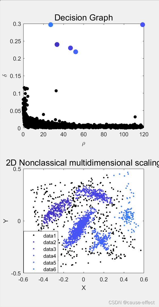
图中看以看出，根据决策图中选中的5个点，聚类结果为5类（黑色的噪声点，不包含在聚类的结果中）。
另外需要注意的一点是，上述程序的输入数据是原始二维数据之间的距离，而不是原始数据，因此可将原始数据处理成相应的距离数据，即可直接利用上述程序。

当然也可以通过修改代码，直接输入原始数据得到聚类结果。代码如下：

    clear all
    close all
    %% 从文件中读取数据
    data_load=dlmread('gauss_data.txt');
    [num,dim]=size(data_load); %数据最后一列是类标签
    data=data_load(:,1:dim-1); %去掉标签的数据
    mdist=pdist(data);         %两两行之间距离
    A=tril(ones(num))-eye(num);
    [x,y]=find(A~=0);
    % Column 1: id of element i, Column 2: id of element j', Column 3: dist(i,j)'
    xx=[x y mdist'];
    ND=max(xx(:,2));
    NL=max(xx(:,1));
    if (NL>ND)
      ND=NL; %% 确保 DN 取为第一二列最大值中的较大者，并将其作为数据点总数
    end
    N=size(xx,1); %% xx 第一个维度的长度，相当于文件的行数（即距离的总个数）
     
    %% 初始化为零
    for i=1:ND
      for j=1:ND
        dist(i,j)=0;
      end
    end
     
    %% 利用 xx 为 dist 数组赋值，注意输入只存了 0.5*DN(DN-1) 个值，这里将其补成了满矩阵
    %% 这里不考虑对角线元素
    for i=1:N
      ii=xx(i,1);
      jj=xx(i,2);
      dist(ii,jj)=xx(i,3);
      dist(jj,ii)=xx(i,3);
    end
     
    %% 确定 dc
    percent=2.0;
    fprintf('average percentage of neighbours (hard coded): %5.6f\n', percent);
     
    position=round(N*percent/100);   %% round 是一个四舍五入函数
    sda=sort(xx(:,3));   %% 对所有距离值作升序排列
    dc=sda(position);
     
    %% 计算局部密度 rho (利用 Gaussian 核)
    fprintf('Computing Rho with gaussian kernel of radius: %12.6f\n', dc);
     
    %% 将每个数据点的 rho 值初始化为零
    for i=1:ND
      rho(i)=0.;
    end
     
    % Gaussian kernel
    for i=1:ND-1
      for j=i+1:ND
         rho(i)=rho(i)+exp(-(dist(i,j)/dc)*(dist(i,j)/dc));
         rho(j)=rho(j)+exp(-(dist(i,j)/dc)*(dist(i,j)/dc));
      end
    end
    %
    % "Cut off" kernel
    %
    %for i=1:ND-1
    %  for j=i+1:ND
    %    if (dist(i,j)<dc)
    %       rho(i)=rho(i)+1.;
    %       rho(j)=rho(j)+1.;
    %    end
    %  end
    %end
    %% 先求矩阵列最大值，再求最大值，最后得到所有距离值中的最大值
    maxd=max(max(dist));
    %% 将 rho 按降序排列，ordrho 保持序
    [rho_sorted,ordrho]=sort(rho,'descend');
    %% 处理 rho 值最大的数据点
    delta(ordrho(1))=-1.;
    nneigh(ordrho(1))=0;
    %% 生成 delta 和 nneigh 数组
    for ii=2:ND
       delta(ordrho(ii))=maxd;
       for jj=1:ii-1
         if(dist(ordrho(ii),ordrho(jj))<delta(ordrho(ii)))
            delta(ordrho(ii))=dist(ordrho(ii),ordrho(jj));
            nneigh(ordrho(ii))=ordrho(jj);
            % 记录 rho 值更大的数据点中与 ordrho(ii) 距离最近的点的编号 ordrho(jj)
         end
       end
    end
     
    %% 生成 rho 值最大数据点的 delta 值
    delta(ordrho(1))=max(delta(:));
     
    %% 决策图
    disp('Generated file:DECISION GRAPH')
    disp('column 1:Density')
    disp('column 2:Delta')
     
    fid = fopen('DECISION_GRAPH', 'w');
    for i=1:ND
       fprintf(fid, '%6.2f %6.2f\n', rho(i),delta(i));
    end
     
    %% 选择一个围住类中心的矩形
    disp('Select a rectangle enclosing cluster centers')
     
    %% 每台计算机，句柄的根对象只有一个，就是屏幕，它的句柄总是 0
    %% >> scrsz = get(0,'ScreenSize')
    %% scrsz =
    %%            1           1        1280         800
    %% 1280 和 800 就是你设置的计算机的分辨率，scrsz(4) 就是 800，scrsz(3) 就是 1280
    scrsz = get(0,'ScreenSize');
     
    %% 人为指定一个位置
    figure('Position',[6 72 scrsz(3)/4. scrsz(4)/1.3]);
     
    %% ind 和 gamma 在后面并没有用到
    for i=1:ND
      ind(i)=i;
      gamma(i)=rho(i)*delta(i);
    end
     
    %% 利用 rho 和 delta 画出一个所谓的“决策图”
    subplot(2,1,1)
    tt=plot(rho(:),delta(:),'o','MarkerSize',5,'MarkerFaceColor','k','MarkerEdgeColor','k');
    title ('Decision Graph','FontSize',15.0)
    xlabel ('\rho')
    ylabel ('\delta')
     
    fig=subplot(2,1,1);
    rect = getrect(fig);
     
    %% getrect 从图中用鼠标截取一个矩形区域， rect 中存放的是
    %% 矩形左下角的坐标 (x,y) 以及所截矩形的宽度和高度
    rhomin=rect(1);
    deltamin=rect(2); %% 作者承认这是个 error，已由 4 改为 2 了!
     
    %% 初始化 cluster 个数
    NCLUST=0;
     
    %% cl 为归属标志数组，cl(i)=j 表示第 i 号数据点归属于第 j 个 cluster
    %% 先统一将 cl 初始化为 -1
    for i=1:ND
      cl(i)=-1;
    end
     
    %% 在矩形区域内统计数据点（即聚类中心）的个数
    for i=1:ND
      if ( (rho(i)>rhomin) && (delta(i)>deltamin))
         NCLUST=NCLUST+1;
         cl(i)=NCLUST;  %% 第 i 号数据点属于第 NCLUST 个 cluster
         icl(NCLUST)=i; %% 逆映射,第 NCLUST 个 cluster 的中心为第 i 号数据点
      end
    end
    fprintf('NUMBER OF CLUSTERS: %i \n', NCLUST);
    disp('Performing assignation')
     
    %assignation
    %% 将其他数据点归类 (assignation)
    for i=1:ND
      if (cl(ordrho(i))==-1)
        cl(ordrho(i))=cl(nneigh(ordrho(i)));
      end
    end
    %halo
    %% 由于是按照 rho 值从大到小的顺序遍历,循环结束后, cl 应该都变成正的值了.
      
    %% 处理光晕点，halo这段代码应该移到 if (NCLUST>1) 内去比较好吧
    for i=1:ND
      halo(i)=cl(i);
    end
    if (NCLUST>1)
         % 初始化数组 bord_rho 为 0,每个 cluster 定义一个 bord_rho 值
      for i=1:NCLUST
        bord_rho(i)=0.;
      end
      % 获取每一个 cluster 中平均密度的一个界 bord_rho
      for i=1:ND-1
        for j=i+1:ND
            %% 距离足够小但不属于同一个 cluster 的 i 和 j
          if ((cl(i)~=cl(j))&& (dist(i,j)<=dc))
            rho_aver=(rho(i)+rho(j))/2.;  %% 取 i,j 两点的平均局部密度
            if (rho_aver>bord_rho(cl(i)))
              bord_rho(cl(i))=rho_aver;
            end
            if (rho_aver>bord_rho(cl(j)))
              bord_rho(cl(j))=rho_aver;
            end
          end
        end
      end
       
    %% halo 值为 0 表示为 outlier
      for i=1:ND
        if (rho(i)<bord_rho(cl(i)))
          halo(i)=0;
        end
      end
    end
     
    %% 逐一处理每个 cluster
    for i=1:NCLUST
      nc=0;  %% 用于累计当前 cluster 中数据点的个数
      nh=0;  %% 用于累计当前 cluster 中核心数据点的个数
      for j=1:ND
        if (cl(j)==i)
          nc=nc+1;
        end
        if (halo(j)==i)
          nh=nh+1;
        end
      end
      fprintf('CLUSTER: %i CENTER: %i ELEMENTS: %i CORE: %i HALO: %i \n', i,icl(i),nc,nh,nc-nh);
    end
     
    cmap=colormap;
    for i=1:NCLUST
       ic=int8((i*64.)/(NCLUST*1.));
       subplot(2,1,1)
       hold on
       plot(rho(icl(i)),delta(icl(i)),'o','MarkerSize',8,'MarkerFaceColor',cmap(ic,:),'MarkerEdgeColor',cmap(ic,:));
    end
    subplot(2,1,2)
    disp('Performing 2D nonclassical multidimensional scaling')
    Y1 = mdscale(dist, 2, 'criterion','metricstress');
    plot(Y1(:,1),Y1(:,2),'o','MarkerSize',2,'MarkerFaceColor','k','MarkerEdgeColor','k');
    title ('2D Nonclassical multidimensional scaling','FontSize',15.0)
    xlabel ('X')
    ylabel ('Y')
    for i=1:ND
     A(i,1)=0.;
     A(i,2)=0.;
    end
    for i=1:NCLUST
      nn=0;
      ic=int8((i*64.)/(NCLUST*1.));
      for j=1:ND
        if (halo(j)==i)
          nn=nn+1;
          A(nn,1)=Y1(j,1);
          A(nn,2)=Y1(j,2);
        end
      end
      hold on
      plot(A(1:nn,1),A(1:nn,2),'o','MarkerSize',2,'MarkerFaceColor',cmap(ic,:),'MarkerEdgeColor',cmap(ic,:));
    end
     
    %for i=1:ND
    %   if (halo(i)>0)
    %      ic=int8((halo(i)*64.)/(NCLUST*1.));
    %      hold on
    %      plot(Y1(i,1),Y1(i,2),'o','MarkerSize',2,'MarkerFaceColor',cmap(ic,:),'MarkerEdgeColor',cmap(ic,:));
    %   end
    %end
    faa = fopen('CLUSTER_ASSIGNATION', 'w');
    disp('Generated file:CLUSTER_ASSIGNATION')
    disp('column 1:element id')
    disp('column 2:cluster assignation without halo control')
    disp('column 3:cluster assignation with halo control')
    for i=1:ND
       fprintf(faa, '%i %i %i\n',i,cl(i),halo(i));
    end

还有一点需要注意的就是，DPC聚类得到的结果图不是原始数据的聚类结果图（看坐标值可以看出来），而是以一种表示方式展示聚类的结果。可以根据聚类得到的数据（分好类的数据）以及聚类中心绘制原始数据聚类结果图，用分好类的数据直接plot即可。

3 总结

DPC作为一种较新的基于密度的聚类算法，得到了广泛的应用，但同时也有人认为DPC只适用于某些数据类型，并非所有情况下效果都好。因此，选择何种聚类算法，还需要根据自己的数据特点及需求，不能盲目选择。