本算法算是本人在学习机器学习过程中的入门算法之一。
该算法实现了纯手工打造,每一行代码都包含原创作者的心血,是算法中的劳斯莱斯,向该算法的原创作者致敬!
参考地址:点击打开
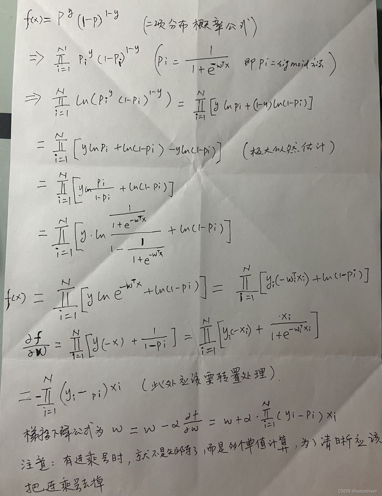
计算较为繁琐,需要用到sigmoid函数和梯度下降算法,算法的步骤主要如下:
- 二项分布概率公式
- 最大似然估计法
- 求导数
- 梯度下降算法和优化
代码:
import numpy as np
import matplotlib.pyplot as plt
def sigmoid(z):
return 1.0/(1+np.exp(-z))
# datas NxD
# labs Nx1
# w Dx1
def weight_update(datas,labs,w,alpha=0.01):
z = np.dot(datas,w) # Nx1
h = sigmoid(z) # Nx1
Error = labs-h # Nx1
w = w + alpha*np.dot(datas.T,Error)
return w
# 随机梯度下降
def train_LR_batch(datas,labs,batchsize=80,n_epoch=2,alpha=0.005):
print("epoch:%d,alpha:%.8f batchsize:%d"%(n_epoch,alpha,batchsize))
N,D = np.shape(datas)
# weight 初始化
w = np.ones([D,1]) # Dx1
N_batch = N//batchsize #取整数
print("n:%d d:%d batchsize:%d"%(N,D,batchsize))
for i in range(n_epoch):
# 数据打乱
rand_index = np.random.permutation(N).tolist()
# 每个batch 更新一下weight
for j in range(N_batch):
print("i:%d j:%d N_batch:%d\r\n"%(i,j,N_batch))
# alpha = 4.0/(i+j+1) +0.01
index = rand_index[j*batchsize:(j+1)*batchsize]
batch_datas = datas[index]
batch_labs = labs[index]
w=weight_update(batch_datas,batch_labs,w,alpha)
error = test_accuracy(datas,labs,w)
print("epoch %d error %.2f%%"%(i,error*100))
return w
def train_LR(datas,labs,n_epoch=2,alpha=0.005):
N,D = np.shape(datas)
w = np.ones([D,1]) # Dx1
# 进行n_epoch轮迭代
for i in range(n_epoch):
w = weight_update(datas,labs,w,alpha)
error_rate=test_accuracy(datas,labs,w)
print("epoch %d error %.3f%%"%(i,error_rate*100))
return w
def test_accuracy(datas,labs,w):
N,D = np.shape(datas)
z = np.dot(datas,w) # Nx1
h = sigmoid(z) # Nx1
lab_det = (h>0.5).astype(np.float)
error_rate=np.sum(np.abs(labs-lab_det))/N
return error_rate
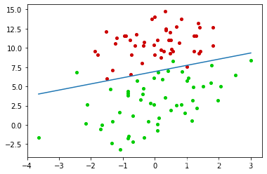
def draw_desion_line(datas,labs,w,name="0.jpg"):
dic_colors={
0:(.8,0,0),1:(0,.8,0)}
# 画数据点
for i in range(2):
index = np.where(labs==i)[0]
sub_datas = datas[index]
plt.scatter(sub_datas[:,1],sub_datas[:,2],s=16.,color=dic_colors[i])
# 画判决线
min_x = np.min(datas[:,1])
max_x = np.max(datas[:,1])
w = w[:,0]
x = np.arange(min_x,max_x,0.01)
y = -(x*w[1]+w[0])/w[2]
plt.plot(x,y)
plt.savefig(name)
def load_dataset(file):
with open(file,"r",encoding="utf-8") as f:
lines = f.read().splitlines()
# 取 lab 维度为 N x 1
labs = [line.split("\t")[-1] for line in lines]
labs = np.array(labs).astype(np.float32)
labs= np.expand_dims(labs,axis=-1) # Nx1
# 取数据 增加 一维全是1的特征
datas = [line.split("\t")[:-1] for line in lines]
datas = np.array(datas).astype(np.float32)
N,D = np.shape(datas)
# 增加一个维度
datas = np.c_[np.ones([N,1]),datas]
return datas,labs
if __name__ == "__main__":
''' 实验1 基础测试数据'''
# 加载数据
file = "testset.txt"
datas,labs = load_dataset(file)
#weights = train_LR(datas,labs,alpha=0.001,n_epoch=800)
weights = train_LR_batch(datas,labs,batchsize=80,alpha=0.001,n_epoch=800)
print(weights)
draw_desion_line(datas,labs,weights,name="test_1.jpg")
训练需要的数据集testset.txt文件:
-0.017612	14.053064	0
-1.395634	4.662541	1
-0.752157	6.538620	0
-1.322371	7.152853	0
0.423363	11.054677	0
0.406704	7.067335	1
0.667394	12.741452	0
-2.460150	6.866805	1
0.569411	9.548755	0
-0.026632	10.427743	0
0.850433	6.920334	1
1.347183	13.175500	0
1.176813	3.167020	1
-1.781871	9.097953	0
-0.566606	5.749003	1
0.931635	1.589505	1
-0.024205	6.151823	1
-0.036453	2.690988	1
-0.196949	0.444165	1
1.014459	5.754399	1
1.985298	3.230619	1
-1.693453	-0.557540	1
-0.576525	11.778922	0
-0.346811	-1.678730	1
-2.124484	2.672471	1
1.217916	9.597015	0
-0.733928	9.098687	0
-3.642001	-1.618087	1
0.315985	3.523953	1
1.416614	9.619232	0
-0.386323	3.989286	1
0.556921	8.294984	1
1.224863	11.587360	0
-1.347803	-2.406051	1
1.196604	4.951851	1
0.275221	9.543647	0
0.470575	9.332488	0
-1.889567	9.542662	0
-1.527893	12.150579	0
-1.185247	11.309318	0
-0.445678	3.297303	1
1.042222	6.105155	1
-0.618787	10.320986	0
1.152083	0.548467	1
0.828534	2.676045	1
-1.237728	10.549033	0
-0.683565	-2.166125	1
0.229456	5.921938	1
-0.959885	11.555336	0
0.492911	10.993324	0
0.184992	8.721488	0
-0.355715	10.325976	0
-0.397822	8.058397	0
0.824839	13.730343	0
1.507278	5.027866	1
0.099671	6.835839	1
-0.344008	10.717485	0
1.785928	7.718645	1
-0.918801	11.560217	0
-0.364009	4.747300	1
-0.841722	4.119083	1
0.490426	1.960539	1
-0.007194	9.075792	0
0.356107	12.447863	0
0.342578	12.281162	0
-0.810823	-1.466018	1
2.530777	6.476801	1
1.296683	11.607559	0
0.475487	12.040035	0
-0.783277	11.009725	0
0.074798	11.023650	0
-1.337472	0.468339	1
-0.102781	13.763651	0
-0.147324	2.874846	1
0.518389	9.887035	0
1.015399	7.571882	0
-1.658086	-0.027255	1
1.319944	2.171228	1
2.056216	5.019981	1
-0.851633	4.375691	1
-1.510047	6.061992	0
-1.076637	-3.181888	1
1.821096	10.283990	0
3.010150	8.401766	1
-1.099458	1.688274	1
-0.834872	-1.733869	1
-0.846637	3.849075	1
1.400102	12.628781	0
1.752842	5.468166	1
0.078557	0.059736	1
0.089392	-0.715300	1
1.825662	12.693808	0
0.197445	9.744638	0
0.126117	0.922311	1
-0.679797	1.220530	1
0.677983	2.556666	1
0.761349	10.693862	0
-2.168791	0.143632	1
1.388610	9.341997	0
0.317029	14.739025	0
anaconda jupyter notebook中的运行结果截图: