Hidden Markov Model - A Tutorial

Hidden Markov Model - A Tutorial

Definition and Representation

* This article assumes that you have a basic knowledge of graph, Markov property and probability theory.

Hidden Markov Model (HMM) is a statistical Markov model in which the system being modeled is assumed to be a Markov process with unobserved (i.e. hidden) states. 

 

A hidden Markov Process, where x is the hidden state and y is the observation . 

A hidden Markov model is characterized by the following parameters

$N$: number of distinct (hidden) states

$M$: number of distinct observations

$\pi$: the prior probability of each state

$\pi=P(x_1=S_i)$

$A$: the transition probability distribution among states (the transition matrix)

$A_{ij}=P(x_{t+1}=S_j|\vert x_t=S_i),\quad 1\le i, j \le N$

$B$: the observation probability distribution for each state (the emission matrix)

 $B_{ik}=P(y_t=S_k\vert x_t=S_i)\quad 1\le i\le N, 1\le k \le M$

As we can see, $N, M$ are the hyperparameter of a hidden Markov model. The other three parameters can be written as: $\lambda=(\pi, A, B)$.

Given appropriate values of $N, M, \pi, A, B$, we can generate a sequence of observations as follows:

• Ÿ       Choose an initial state  $x_1=S_i$ according to the initial state distribution $\pi$
• Ÿ       Generate observation $y_t$ according to $B$
• Ÿ       Transit to a new state $x_{t+1}$ according to $A$
• Ÿ       Repeat until we have $T$ states

The transfer and emission probability among states and observations

Where Can It Be Used?

HMMs can be applied in many fields where the goal is to recover a data sequence that is not immediately observable (but other data that depend on the sequence are). In robotics/human-robot interaction, common usages include: speech recognition, synthesis and tagging, natural language analysis, machine translation, handwriting recognition, time series analysis, activity recognition, sequence classification, etc.

The Three Problem in HMM and Algorithms

We already have the mathematical representation of hidden Markov model. In order to use it in real-world application, there are three basic problems to solve about HMM: the evaluation problem, the hidden-state discover problem, and the parameter optimization (training) problem. In this section, we will specify the three problems, their corresponding algorithm, complexity, and applications.

Problem 1: Evaluation

Formulation: Given a HMM model $(\pi, A, B)$ and a sequence of observations $Y=y_1, y_2, \cdots, y_T$ , compute the probability that the observation is produced by this model.

The evaluation problem can be considered as a scoring of how well a given model matches an observation sequence. It can be used to evaluate models and selecting the model best matches the observations.

The most straightforward way to calculate the required probability is to enumerate every possible state sequence of length $T$. We can prove that the cost of doing so is $2TN^2$, which is computationally unfeasible. An effective solution to this problem is dynamic programming, or in its particular name: the forward-backward procedure, where we can memorizes the probability of partial sequence for further computation. The forward procedure propagate goes from $t=1$ to $t=T$ and the backward procedure do it the other way. But the processes are similar and the results are the same. 

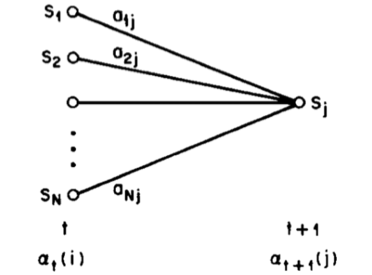
Take the forward procedure for example, we introduce the forward variable $\alpha_t(i)$, which indicates the probability of the partial observation sequence from 1 to t. with state $i$ at time $t$:

 $a_t(i)=P(y_1, \cdots, y_t, x_t=S_i\vert \lambda)$

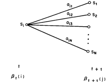
Similarly, we can define the backward variable $\beta_t(i)$:

 $\beta_t(i)=P(y_{t+1},\cdots y_T\vert x_t=S_i, \lambda)$

i.e. the probability of the partial observation sequence from t+1 to the end, with state $i$ at time t.

The algorithm can be summarized as follows:

The Forward-Backward Procedure

The Forward Procedure

1. Initialization

$a_1{i}=\pi_iB_{iy_1}\quad1\le i\le N$

2. Induction

    For $t=1:T-1$, compute:

 $a_{t+1}(i)=(\sum_{j=1}^N \alpha_t(j)A_{ji})B_{iy_{t+1}}, \quad 1\le i \le N$

3. Termination

$P(Y\vert\lambda)=\sum_{i=1}^N\alpha_T(i)$

The Backward Procedure

1. Initialization

$\beta_T{i}=1\quad1\le i\le N$

2. Induction

    For $t=T-1:1$, compute:

$\beta_t(i)=\sum_{j=1}^NA_{ij}B_{iy_{t+1}}\beta_{t+1}(j),\quad 1\le i\le N$

3. Termination

$P(Y\vert\lambda)=\sum_{i=1}^N\beta_1(i)\pi_i$

 The cost of Forward-Backward Procedure is .

 

     Forward                              Backward

Problem 2: Hidden State Discovery

Formulation: Given a HMM model $(\pi, A, B)$ and a sequence of observations $Y=y_1, y_2, \cdots, y_T$, choose an “optimal” sequence of states $x_1, x_2, \cdots, x_T$ which best matches the observations.

The hidden state discovery is a typical task in learning about the structure of the model, to find optimal state sequence in applications such as text translation and continuous speech recognition.

Unlike the evaluation problem, this problem doesn’t have an exact solution, because there are several reasonable optimality criteria that can be used to retrieve the hidden states. E.g. choosing the states based on individually most likelihood,maximize the expected number of correct pairs of states or triples of states, etc. However, the most widely used criterion is to find the single best state sequence, i.e. to maximize $P(X|Y, \lambda)$, namely theViterbi algorithm.

To do this, define quantity $\delta_t(i)$, which is the highest probability along a single path at time t, which accounts for the first t observations and ends in state $i$:

 $\delta_t(i)=\max\limits_{x_{1:t-1}} P(x_1, \cdots, x_t=S_i, y_1, \cdots, y_t \vert \lambda)$

In order to retrieve the state sequence, we need another array to record the argument of each maximization. We call this array $\psi_t(i)$. The pseudocode for Viterbi algorithm is:

Viterbi Algorithm

Initialization

$\delta_1(i)=\pi_i b_{iy_1}, \quad 1\le j \le N$

$\psi_1(i)=0, \quad 1 \le j \le N$

Recursion

For $t=2:T$ do:

$\delta_t(j) = \max\limits_{1\le i \le N} \delta_{t-1}(i)A_{ij}B_{jy_t}, \quad 1\le j\le N$

$\psi_t(j) = \arg \max\limits_{1\le i\le N} \delta_{t-1}(i)A_{ij}, \quad 1\le j \le N$ 

Termination

$P^*=\max\limits_{1\le i \le N}\delta_T(i)$

$x^*_T = \arg\max\limits_{1\le i\le N}\delta_T(i)$

Path backtracking

For $t=T-1:1$ do:

 $x^*_t=\psi_{t+1}(x^*_{t+1})$

We can see that the Viterbi algorithm is similar in implementation to the forward calculation.

Problem 3: Training

Formulation: Given an observation sequence $Y=y_1, y_2, \cdots, y_T$, find the model parameter $\lambda=(\pi, A, B)$ that maximize $P(Y\vert\lambda)$

The training problem is one of the most important problem for HMM applications, since it allows us to optimally adapt model parameters to fit the training data, which can be later used for prediction and classification.

Unlike the above problems, there is no analytical way of estimating the model parameters. However, we can use an iterative method, while in each iteration $P(Y\vert\lambda)$ is locally maximized. This is called the Baum-Welch methodfor HMM, or in a more generally case the Expectation-Maximization (EM) algorithm. There are other training methods, such as gradient descent. But we will focus of the most commonly used iterative procedure method in this article.

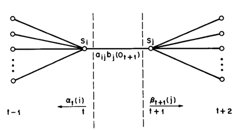
In order to describe the procedure, first define $\xi_t(i, j)$, the probability of being in state $S_i$ at time $t$ and state $S_j$ at time $t+1$:

$\xi_t(i,j)=P(x_t=S_i, x_{t+1}=S_j\vert Y, \lambda)=\frac{\alpha_t(i)A_{ij}B_{jy_{t+1}}\beta_{t+1}(i)}{P(Y\vert \lambda)}=\frac{\alpha_t(i)A_{ij}B_{jy_{t+1}}\beta_{t+1}(i)}{\sum_{i=1}^N\sum_{j=1}^N\alpha_t(i)A_{ij}B_{jy_{t+1}}\beta_{t+1}(i)}$

Also, define  as the probability of begin in state $i$ at time t: 

 $\gamma_t(i)=P(x_t=S_i\vert Y, \lambda)=\frac{\alpha_t(i)\beta_t(i)}{P(Y\vert\lambda)}=\frac{\alpha_t(i)\beta_t(i)}{\sum_{i=1}^N\alpha_t(i)\beta_t(i)}$

It is not hard to see that $\gamma_t(i)=\sum_{j=1}^N\xi_t(i,j)$. The summation of $\gamma_t(i)$ over time can be interpreted as the expected number of times that state $i$  is visited, or the expected number of transitions made from state $i$; While the summation of $\xi_t(i,j)$ over time, can be interpreted as the expected number transitions from state $i$ to state $j$.

The Baum-Welch algorithm can be summarized as:

Baum-Welch Algorithm (EM) for training HMM

(E-step)

Compute forward and backward probabilities $\alpha_t, \beta_t, \gamma_t, \xi_t$ and $P(Y\vert\lambda)$ 

(M-step)

Update parameters:

 $\pi_i=\gamma_1(i), \quad A_{ij}=\frac{\sum_{t=1}^{T-1}\xi_t(i,j)}{\sum_{t=1}^{T-1}\gamma_t(i,j)}, \quad B_{ik}=\frac{\sum_{t=1, s.t y_t=k}^{T}\gamma_t(i,j)}{\sum_{t=1}^{T}\gamma_t(i,j)}$

Repeat until converge.

Train with Multiple Observation Sequences

In order to achieve reliable model parameters, most of the time we have multiple observation sequences for training a HMM. We can simply modified our method to learn a model using more than one sequences at the same time.

We denote the set of K observation sequences as $\mathbf{Y}={Y^1, Y^2, \cdots, Y^K}$, the overall probability to maximize becomes:

 $P(\mathbf{Y}\vert\lambda)=\prod_{k=1}^K P(Y^k\vert\lambda)$

Then the update formulas in Baum-Welch becomes:

$\pi_i=\sum_{k=1}^K\gamma_1^k(i), \quad A_{ij}=\frac{\sum_{k=1}^K\sum_{t=1}^{T-1}\xi_t(i,j)}{\sum_{k=1}^K\sum_{t=1}^{T-1}\gamma_t(i,j)}, \quad B_{ik}=\frac{\sum_{k=1}^K\sum_{t=1, s.t y_t=k}^{T}\gamma_t(i,j)}{\sum_{k=1}^K\sum_{t=1}^{T}\gamma_t(i,j)}$

Implementation Detail: Scaling vs Logarithm

One tricky problem in the implementation of HMM algorithms is underflow. The probabilities consist of multiplications of a series of small elements, thus their value head exponentially to zero. In order to avoid such underflow problem, there are generally two way to perform the algorithms effectively: scaling or compute the log-likelihood instead.

Scaling

To avoid underflow, the probabilities need to be rescaled every time after computation. More specifically, we need to normalize $\alpha$ and $\beta$ every time after the update:

 $c_t=\frac{1}{\sum_{i=1}^N\alpha_t(i)}, \quad \hat{\alpha}_t(i)=c_t\alpha_t(i)$

 $d_t=\frac{1}{\sum_{i=1}^N\beta_t(i)}, \quad \hat{\beta}_t(i)=d_t \beta_t(i)$

Then treat $\hat{\alpha}_t(i)$ and $\hat{\beta}_t(i)$ normally as $\alpha_t(i)$ and $\beta_t(i)$ during computation.

Take Logarithm

Another method to avoid underflow is to take logarithm of the probabilities and variables during the computation. The induction process has the form of: 

$\log \alpha_{t+1}(j)=\log \exp(\log \alpha_t(i) + \log A_{ij})+\log B_{jy_{t+1}}$

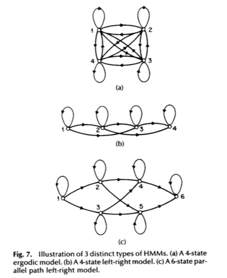
Variants of HMM

There are several special types of hidden Markov models. In the previous part, we assumes the most general case: an ergodic/fully connected HMM, in which every state of the model could be reached from every other state (in a finite number of steps. For some applications, we will be using some special types of HMM. The left-right model or a Bakis model is one example, where the state index can only increases or stay the same as time goes on. In other words, we have $\pi_1=1, \pi_i=0$ for $\forall i>1$; $A_{ij}$ if and only if $i\le j$.

An Example: Gesture Recognition using HMM

One example of HMM is to gesture (hand movement pattern) recognition. The input could be a sequence of data indicating hand movement (e.g. IMU sensor reading) over time. We can train a HMM for each gesture, using single or multiple data sequences. Then we can predict the label of any observation sequence by comparing its log-likelihood under each gesture’s model. 

Note that the raw observations are usually multi-dimensional and continuous, in order to apply the hidden Markov model to the continuous data, we need to discretize the raw observation (e.g. using clustering method) before training a HMM.

References

1. L. R. Rabiner, "A tutorial on hidden Markov models and selected applications in speech recognition," in Proceedings of the IEEE, vol. 77, no. 2, pp. 257-286, Feb 1989.
2. Xiaolin Li, M. Parizeau and R. Plamondon, "Training hidden Markov models with multiple observations-a combinatorial method," in IEEE Transactions on Pattern Analysis and Machine Intelligence, vol. 22, no. 4, pp. 371-377, Apr 2000.