Hidden Markov Model (HMM) 详细推导及思路分析

往期文章链接目录

Before reading this post, make sure you are familiar with the EM Algorithm and decent among of knowledge of convex optimization. If not, please check out my previous post

• EM Algorithm

• convex optimization primal and dual problem

Let’s get started!

Conditional independence

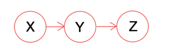
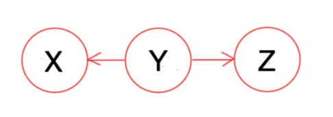
$A$ and $B$ are conditionally independent given $C$ if and only if, given knowledge that $C$ occurs, knowledge of whether $A$ occurs provides no information on the likelihood of $B$ occurring, and knowledge of whether $B$ occurs provides no information on the likelihood of $A$ occurring.

Formally, if we denote conditional independence of $A$ and $B$ given $C$ by $(A\perp \!\!\!\perp B)\mid C$, then by definition, we have

$(A\perp \!\!\!\perp B)\mid C\quad \iff \quad P(A, B\mid C)= P(A\mid C) \cdot P(B\mid C)$

Given the knowledge that $C$ occurs, to show the knowledge of whether $B$ occurs provides no information on the likelihood of $A$ occurring, we have

$\begin{aligned} P(A | B ,C) &=\frac{P(A , B , C)}{P(B , C)} \\ &=\frac{P(A , B | C) \cdot P(C)}{P(B , C)} \\ &=\frac{P(A | C) \cdot P(B | C) \cdot P(C)}{P(B | C) \cdot P(C)} \\ &=P(A | C) \end{aligned}$

Two classical cases where $X$ and $Z$ are conditionally independent

Case 1 :

From the above directed graph, we have $P(X,Y,Z) = P(X)\cdot P(Y|X)\cdot P(Z|Y)$. Hence we have

$\begin{aligned} P(Z|X,Y) &= \frac{P(X,Y,Z)}{P(X,Y)}\\ &= \frac{P(X)\cdot P(Y|X)\cdot P(Z|Y)}{P(X)\cdot P(Y|X)}\\ &= P(Z|Y) \end{aligned}$

Therefore, $X$ and $Z$ are conditionally independent.

Case 2 :

From the above directed graph, we have $P(X,Y,Z) = P(Y)\cdot P(X|Y) \cdot P(Z|Y)$. Hence we have

$\begin{aligned} P(Z|X,Y) &= \frac{P(X,Y,Z)}{P(X,Y)}\\ &= \frac{P(Y)\cdot P(X|Y) \cdot P(Z|Y)}{P(Y)\cdot P(X|Y)}\\ &= P(Z|Y) \end{aligned}$

Therefore, $X$ and $Z$ are conditionally independent.

Settings of the Hidden Markov Model (HMM)

The HMM is based on augmenting the Markov chain. A Markov chain is a model that tells us something about the probabilities of sequences of random variables, states, each of which can take on values from some set. A Markov chain makes a very strong assumption that if we want to predict the future in the sequence, all that matters is the current state.

To put it formally, suppose we have a sequence of state variables $z_1, z_2, ..., z_n$. Then the Markov assumption is

$p(z_n | z_1z_2...z_{n-1}) = p(z_n | z_{n-1})$

A Markov chain is useful when we need to compute a probability for a sequence of observable events. However, in many cases the events we are interested in are hidden. For example we don’t normally observe part-of-speech (POS) tags in a text. Rather, we see words, and must infer the tags from the word sequence. We call the tags hidden because they are not observed.

A hidden Markov model (HMM) allows us to talk about both observed events (like words that we see in the input) and hidden events (like part-of-speech tags) that we think of as causal factors in our probabilistic model. An HMM is specified by the following components:

• A sequence of hidden states $z$, where $z_k$ takes values from all possible hidden states $Z = \{1,2,..,m\}$.

• A sequence of observations $x$, where $x = (x_1, x_2, ..., x_n)$. Each one is drawn from a vocabulary $V$.

• A transition probability matrix $A$, where $A$ is an $m \times m$ matrix. $A_{ij}$ represents the probability of moving from state $i$ to state $j$: $A_{ij} = p(z_{t+1}=j| z_t=i)$, and $\sum_{j=1}^{m} A_{ij} = 1$ for all $i$.

• An emission probability matrix $B$, where $B$ is an $m \times |V|$ matrix. $B_{ij}$ represents the probability of an observation $x_j$ being generated from a state $i$: $B_{ij} = P(x_t = V_j|z_t = i)$

• An initial probability distribution $\pi$ over states, where $\pi = (\pi_1, \pi_2, ..., \pi_m)$. $\pi_i$ is the probability that the Markov chain will start in state $i$. $\sum_{i=1}^{m} \pi_i = 1$.

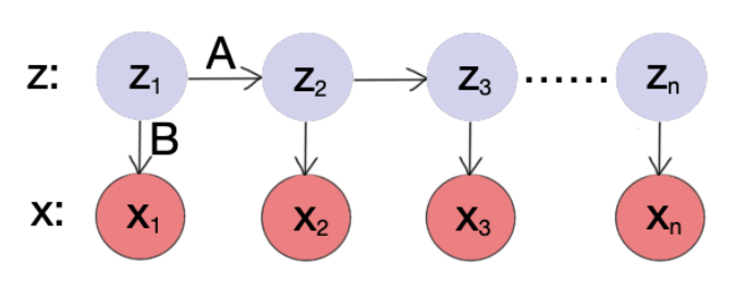
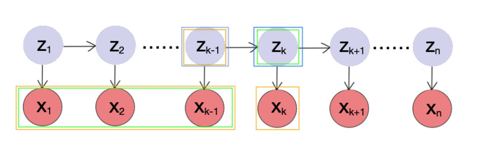
Given a sequence $x$ and the corresponding hidden states $z$ (like one in the picture above), we have

$P(x, z|\theta) = p(z_1) \cdot [p(z_2|z_1)\cdot p(z_3|z_2)\cdot ... \cdotp(z_n|z_{n-1})] \cdot [p(x_1|z_1)\cdot p(x_2|z_2)\cdot ... \cdot p(x_n|z_n)] \tag 0$

We get $p(z_1)$ from $\pi$, $p(z_{k+1}|z_k)$ from $A$, and $p(x_k|z_k)$ from $B$.

Useful probabilities $p(z_k | x)$ and $p(z_{k+1}, z_k | x)$

$p(z_k | x)$ and $p(z_{k+1}, z_k | x)$ are useful probabilities and we are going to use them later.

Intuition: Once we have a sequence $x$, we might be interested in find the probability of any hidden state $z_k$, i.e., find probabilities $p(z_k =1| x), p(z_k =2| x), ..., p(z_k =m| x)$. we have the following

$\begin{aligned} p(z_k | x) &= \frac{p(z_k, x)}{p(x)} & & (1)\\ &\propto p(z_k, x) & & (2)\\ \end{aligned}$

Note that from $(1)$ to (2), since $p(x)$ doesn’t change for all values of $z_k$, $p(z_k | x)$ is proportional to $p(z_k, x)$.

$\begin{aligned} p(z_k=i, x) &= p(z_k=i, x_{1:k}, x_{k+1:n}) \\ &= p(z_k=i, x_{1:k}) \cdot p(x_{k+1:n}|z_k=i, x_{1:k}) & & (3)\\ &= p(z_k=i, x_{1:k}) \cdot p(x_{k+1:n}|z_k=i) & & (4.1) \\ &= \alpha_k(z_k=i) \cdot \beta_k(z_k=i) &&(4.11)\\ \end{aligned}$

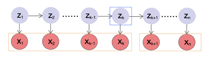
From the above graph, we see that the second term $(3)$ is the 2nd classical cases. So $x_{k+1:n}$ and $x_{1:k}$ are conditionally independent. This is why we can go from $(3)$ to $(4.1)$. We are going to use the Forward Algorithm to compute $p(z_k, x_{1:k})$, and Backward Algorithm to compute $p(x_{k+1:n}|z_k)$ later.

We denote $p(z_k, x_{1:k})$ by $\alpha_k(z_k)$ and $p(x_{k+1:n}|z_k)$ by $\beta_k(z_k)$.

After we know how to calculate these two terms separately, we can calculate $p(z_k | x)$ easily by introducing a normalization term. That is,

$\begin{aligned} p(z_k = i | x) &= \frac{p(z_k = i, x)}{\sum_{j=1}^m p(z_k = j, x)} \\ &= \frac{\alpha_k(z_k=i)\beta_k(z_k=i)}{\sum_{j=1}^{m} \alpha_k(z_k=j)\beta_k(z_k=j)} && (4.2) \end{aligned}$

where $\sum_j^m p(z_k = j, x)$ is the normalization term which makes $p(z_k = 1, x)$ take values between $0$ and $1$ for all $z_k$.

Similarly, we are also interested in finding $p(z_{k+1}, z_k | x)$, where

$p(z_{k+1}, z_k | x) \propto p(z_{k+1}, z_k, x)$

By using the property of conditional independence, we have

$\begin{aligned} p(z_{k+1}=j, z_k=i, x) &= p(z_k=i, z_{k+1}=j, x_{1:k}, x_{k+1}, x_{k+2:n}) \\ &= p(z_k=i, x_{1:k}) \cdot p(x_{k+2:n)|z_{k+1}=j}) \cdot p(z_{k+1}=j|z_{k}=i) \cdot p(x_{k+1}| z_{k+1}=j) && (4.3)\\ &= \alpha_k(z_k=i) \cdot \beta_{k+1}(z_{k+1}=j) \cdot p(z_{k+1}=j|z_{k}=i) \cdot p(x_{k+1}| z_{k+1}=j) && (4.4) \\ \end{aligned}$

Note that we can find the third and the forth term from the transition probability matrix and the emission probability matrix. Again, we can calculate $p(z_{k+1}, z_k | x)$ simply by introducing a normalization term. That is,

$\begin{aligned} p(z_{k+1}=s, z_k=r | x) &= \frac{p(z_{k+1}=s, z_k=r, x)}{\sum_{i=1}^{m} \sum_{j=1}^{m} p(z_{k+1}=j, z_k=i, x)} \\ &= \frac{\alpha_k(z_k=r) \cdot \beta_{k+1}(z_{k+1}=s) \cdot p(z_{k+1}=s|z_{k}=r) \cdot p(x_{k+1}| z_{k+1}=s)}{\sum_{i=1}^{m} \alpha_k(z_k=i) \cdot \beta_{k+1}(z_{k+1}=j) \cdot p(z_{k+1}=j|z_{k}=i) \cdot p(x_{k+1}| z_{k+1}=j)} && (4.42) \end{aligned}$

Remark

• We denote

  $\gamma_k(i) = p(z_k = i | x) = \frac{p(z_k=i, x)}{p(x)} \tag{4.43}$

• We denote

  $\xi_k(i,j) = p(z_{k+1}=j, z_k=i | x) = \frac{p(z_{k+1}=j, z_k=i, x)}{p(x)} \tag{4.44}$

Three fundamental problems of HMM

Problem 1 (Likelihood): Given an observation sequence $x$ and parameters $\theta = (A, B, \pi)$, determine the likelihood $p(x|\theta)$.

Problem 2 (Learning): Given an observation sequence $x$, learn the parameters $\theta = (A, B, \pi)$.

Problem 3 (Inference): Given an observation sequence $x$ and parameters $\theta = (A, B, \pi)$, discover the best hidden state sequence $z$.

Problem 1 (Likelihood)

Goal: Given an observation sequence $x$ and parameters $\theta = (A, B, \pi)$, determine the likelihood $p(x|\theta)$.

Naive Way:

From $(0)$, we have already know how to compute $P(x, z|\theta)$, so we can compute $p(x|\theta)$ by summing all possible sequence $z$:

$p(x|\theta) = \sum_z P(x, z|\theta) \cdot p(z|\theta)$

This method is not applicable since there are $m^n$ ways of combinations of sequence $z$. So we introduce the following two algorithm: Forward Algorithm and Backward Algorithm.

Forward Algorithm

• Goal: Compute $p(z_k, x_{1:k})$, given $\theta = (A, B, \pi)$.

From the picture above, it’s natural to compute $p(z_k, x_{1:k})$ by dynamic programming (DP). That is, to calculate it in terms of $p(z_{k-1}, x_{1:k-1})$:

$\begin{aligned} p(z_k , x_{1:k}) &= \sum_{z_{k-1}} p(z_k, z_{k-1}, x_{1:k-1}, x_k) & & (5)\\ &= \sum_{z_{k-1}} p(z_{k-1}, x_{1:k-1}) \cdot p(z_k, x_k|z_{k-1}, x_{1:k-1}) & & (6)\\ &= \sum_{z_{k-1}} p(z_{k-1}, x_{1:k-1}) \cdot p(z_k|z_{k-1}, x_{1:k-1}) \cdot p(x_k|z_k, z_{k-1}, x_{1:k-1}) & & (7)\\ &= \sum_{z_{k-1}} p(z_{k-1}, x_{1:k-1}) \cdot p(z_k|z_{k-1}) \cdot p(x_k|z_k) & & (8)\\ \end{aligned}$

Ramark:

• From $(6)$ to $(7)$, we use the fact that $p(b,c|a) = p(b|a) \cdot p(c|a,b)$.

• From $(7)$ to $(8)$, we use the conditional independence, which is visualized in the picture above.

• We denote $p(z_k , x_{1:k})$ by $\alpha_k(z_k)$, so

  $\alpha_k(z_k) = p(z_k , x_{1:k}) = \sum_{z_{k-1}} \alpha_{k-1}(z_{k-1}) \cdot p(z_k|z_{k-1}) \cdot p(x_k|z_k) \tag 9$

• In equation $(9)$, the term $p(z_k|z_{k-1})$ is the transition probability from state $z_{k-1}$ to state $z_{k}$; the term $p(x_k|z_k)$ is the emission probability of observing $x_k$ given state $z_k$.

• $\alpha_1(z_1=q) = p(z_1=q, x_1) = \pi_q \cdot p(x_1 | z_1 = q)$, where $p(x_1 | z_1 = q)$ is an emmission probability.

Knowing how to compute $p(z_k , x_{1:k})$ recurssively, we have

$p(x|\theta) = p(x_{1:n}|\theta) = \sum_{z_n} p(z_n, x_{1:n}) = \sum_{z_n} \alpha_n(z_n) = \sum_{q=1}^{m} \alpha_n(z_n=q)$

Backward Algorithm

• Goal: Compute $p(x_{k+1:n} | z_k)$, given $\theta = (A, B, \pi)$.

Again, we are going to use DP to compute $p(x_{k+1:n} | z_k)$ in terms of $p(x_{k+2:n} | z_{k+1})$:

$\begin{aligned} p(x_{k+1:n} | z_k) &= \sum_{z_{k+1}} p(x_{k+1}, x_{k+2:n}, z_{k+1} | z_k) \\ &= \sum_{z_{k+1}} p(x_{k+2:n}, z_{k+1}| z_k) \cdot p(x_{k+1}| z_k, x_{k+2:n}, z_{k+1}) \\ &= \sum_{z_{k+1}} p(z_{k+1}|z_k) \cdot p(x_{k+2:n}|z_{k+1}, z_k) \cdot p(x_{k+1} | z_k, x_{k+2:n}, z_{k+1}) && (10)\\ &= \sum_{z_{k+1}} p(x_{k+2:n}|z_{k+1}) \cdot p(z_{k+1}|z_k) \cdot p(x_{k+1}|z_{k+1}) && (11)\\ \end{aligned}$

Ramark:

• From $(10)$ to $(11)$, we use the conditional independece similar to the one in forward algorithm.

• We denote $p(x_{k+1:n} | z_k)$ by $\beta_k(z_k)$, so

  $\beta_k(z_k) = p(x_{k+1:n} | z_k) = \sum_{z_{k+1}} p(x_{k+2:n}|z_{k+1}) \cdot p(z_{k+1}|z_k) \cdot p(x_{k+1}|z_{k+1}) \tag {12}$

• In equation $(12)$, the term $p(z_{k+1}|z_k)$ is the transition probability from state $z_{k}$ to state $z_{k+1}$; the term $p(x_{k+1}|z_{k+1})$ is the emission probability of observing $x_{k+1}$ given state $z_{k+1}$.

• $\beta_n(z_n) = 1$.

Knowing how to compute $p(x_{k+1:n} | z_k)$ recursively, we have

$\begin{aligned} p(x|\theta) &= \sum_{z_1} p(x, z_1) = \sum_{z_1} p(x | z_1) \cdot p(z_1) \\ &= \sum_{z_1} p(x_1, x_{1+1:n} | z_1) \cdot p(z_1) \\ &= \sum_{z_1} p(x_1 | z_1) \cdot p(x_{1+1:n}|z_1, x_1) \cdot p(z_1) &&(13)\\ &= \sum_{z_1} p(x_1 | z_1) \cdot p(x_{1+1:n}|z_1) \cdot p(z_1) &&(14)\\ &= \sum_{z_1} p(x_1 | z_1) \cdot \beta_1(z_1) \cdot p(z_1) \\ &= \sum_{q=1}^m \beta_1(z_1=q) \cdot p(x_1 | z_1=q) \cdot \pi_q \end{aligned}$

From $(13)$ to $(14)$, we use the conditional independence. To make it clean, I didn’t include $\theta$ in the above derivation, but keep in mind $x$ is conditioned on $\theta$.

Problem 2 (Learning)

Goal: Given an observation sequence $x$, learn the parameters $\theta = (A, B, \pi)$.

Given that the hidden states are unknown, it’s natural to use the EM Algorithm to solve parameters. Remind that the EM Algorithm consists of two steps:

• An expectation (E) step, which creates a function $Q(\theta, \theta_i)$ for the expectation of the log-likelihood $\log p(x,z|\theta)$ evaluated using the current conditional distribution of $z$ given $x$ and the current estimate of the parameters $\theta_i$, where

$\begin{aligned} Q(\theta, \theta_i) &= E_{z \sim P(z|x,\theta_i)}[\log p(x,z|\theta)] \\ &= \sum_z P(z|x,\theta_i) \cdot \log p(x,z|\theta) \\ \end{aligned}$

• A maximization (M) step, which computes parameters maximizing the expected log-likelihood $Q(\theta, \theta_i)$ found on the $E$ step and then update parameters to $\theta_{i+1}$.

We fist initialize parameters $\theta_0 = (A_0, B_0, \pi_0)$

E Step:

We are going to construct $Q(\theta, \theta_i)$.

$\begin{aligned} Q(\theta, \theta_i) &= E_{z \sim P(z|x,\theta_i)}[\log p(x,z|\theta)] \\ &= \sum_z P(z|x,\theta_i) \cdot \log p(x,z|\theta) \\ &= \log p(x,z|\theta) \cdot \frac{p(x,z|\theta_i)}{p(x|\theta_i)} &&(15)\\ &\propto \log p(x,z|\theta) \cdot p(x,z|\theta_i) &&(16)\\ \end{aligned}$

Since we know $x$ and $\theta_i$, $p(x|\theta_i)$ is a constant and therefore we can write from $(15)$ to $(16)$. In the earlier section “Settings of the Hidden Markov Model” of the post, we deduce that

$P(x, z|\theta) = p(z_1) \cdot [p(z_2|z_1)\cdot p(z_3|z_2)\cdot ... \cdotp(z_n|z_{n-1})] \cdot [p(x_1|z_1)\cdot p(x_2|z_2)\cdot ... \cdot p(x_n|z_n)]$

So we can formulate $Q(\theta, \theta_i)$ as

$\begin{aligned} Q(\theta, \theta_i) &= \sum_z \left( \log \pi_{z_i} + \sum_{t=1}^{n-1} \log p(z_{t+1}|z_t) + \sum_{t=1}^{n} \log p(x_n|z_n)\right) \cdot p(x,z|\theta_i) \\ &= \sum_z \log \pi_{z_i} \cdot p(x,z|\theta_i) + \sum_z \sum_{t=1}^{n-1} \log p(z_{t+1}|z_t) \cdot p(x,z|\theta_i) + \sum_z \sum_{t=1}^{n} \log p(x_t|z_t) \cdot p(x,z|\theta_i) \\ \end{aligned}$

M Step:

We are going to maximize $Q(\theta, \theta_i)$ and update $\theta_{i+1}$.

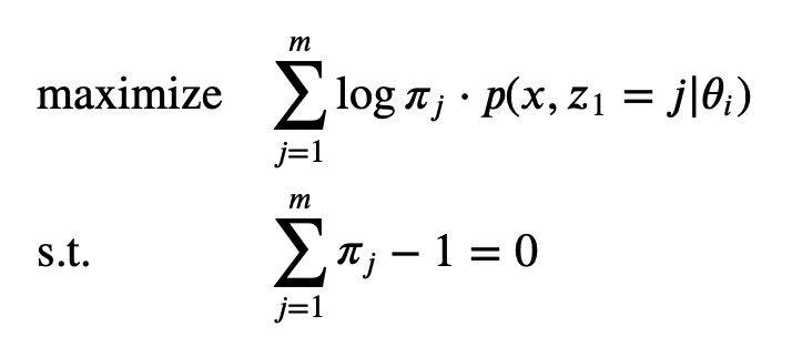
Note that we write $Q(\theta, \theta_i)$ as the sum of three terms. The first therm is related to $\pi$, the second term is related to $A$, and the third term is related to $B$. Therefore we can maximize each term separately.

We can write the first term as

$\sum_z \log \pi_{z_i} \cdot p(x,z|\theta_i) = \sum_{j=1}^m \log \pi_j \cdot p(x, z_1 = j|\theta_i)$

under the constraint $\sum_{j=1}^m \pi_j = 1$. Clearly, this is a convex optimization problem:

The Lagrangian $L$ associated with the problem is

$L(\pi, v) = \sum_{j=1}^m \log \pi_j \cdot p(x, z_1 = j|\theta_i) + v \cdot (\sum_{j=1}^m \pi_j - 1)$

Note that any pair of primal and dual optimal points must satisfy the KKT conditions. So we use one KKT property that the gradient must vanish at the optimal point to find $\pi$. This might not be the optimal $\pi$ since “any pair of primal and dual optimal points must satisfy the KKT conditions” doesn’t imply that a point satisfying the KKT conditions is the optimal.

$\begin{aligned} \frac{\partial L}{\partial \pi_j} = p(x, z_1=j|\theta_i) \cdot \frac{1}{\pi_j} + v & = 0 \\ p(x, z_1=j|\theta_i) + v \cdot \pi_j & = 0 \\ \pi_j & = \frac{-p(x, z_1=j|\theta_i)}{v} & & (17)\\ \end{aligned}$

By setting $\frac{\partial L}{\partial \pi_j} = 0$ for all $j$, we have

$\begin{aligned} \sum_{j=1}^m p(x, z_1=j|\theta_i) + v \cdot \sum_{j=1}^m \pi_j &= 0 \\ p(x|\theta_i) + v &= 0\\ v &= - p(x|\theta_i) && (18)\\ \end{aligned}$

By plugging $(18)$ into $(17)$, we have

$\pi_j = \frac{-p(x, z_1=j|\theta_i)}{v} = \frac{p(x, z_1=j|\theta_i)}{p(x|\theta_i)} = \gamma_1(j)$.

In the similar way, we can write the second term as

$\sum_z \sum_{t=1}^{n-1} \log p(z_{t+1}|z_t) \cdot p(x,z|\theta_i) = \sum_{j=1}^m \sum_{k=1}^m \sum_{t=1}^{n-1} \log p(z_{t+1}=k|z_t=j) \cdot p(x,z_t=j, z_{t+1}=k|\theta_i) \\ \sum_z \sum_{t=1}^{n} \log p(x_t|z_t) \cdot p(x,z|\theta_i) = \sum_{j=1}^m \sum_{t=1}^n \log p(x_t|z_t=j) \cdot p(x,z_t=j|\theta_i)$

with seperate constraints

$\sum_{k=1}^m p(z_{t+1}=k|z_t=j) = 1, \\ \sum_{j=1}^m p(x_t|z_t=j) = 1$

We can solve for optimal parameters similar to solving for $\pi$. After we set the gradient of corresponding Lagrangian to $0$, we have

$\begin{aligned} A_{jk} &= p(z_{t+1}=k|z_t=j) \\ &= \frac{\sum_{t=1}^{n-1} p(x, z_t=j, z_{t+1}=k|\theta_i)}{\sum_{t=1}^{n-1} p(x, z_t=j|\theta_i)} \\ &= \frac{\sum_{t=1}^{n-1} p(x, z_t=j, z_{t+1}=k|\theta_i)/ p(x|\theta_i)}{\sum_{t=1}^{n-1} p(x, z_t=j|\theta_i)/p(x|\theta_i)} \\ &= \frac{\sum_{t=1}^{n-1} \xi_t(jk)}{\sum_{t=1}^{n-1} \gamma_t(j)} &&(19)\\\\ B_{jk} &= p(x_t= V_k|z_t=j) \\ &= \frac{\sum_{t=1}^{n-1} p(x, z_t=j|\theta_i)\cdot I(x_t= V_k)}{\sum_{t=1}^{n-1} p(x, z_t=j | \theta_i)} \\ &= \frac{\sum_{t=1}^{n-1} p(x, z_t=j|\theta_i)/ p(x|\theta_i) \cdot I(x_t= V_k)}{\sum_{t=1}^{n-1} p(x, z_t=j | \theta_i)/ p(x|\theta_i)} \\ &= \frac{\sum_{t=1}^{n-1} \gamma_t(j) \cdot I(x_t=V_k)}{\sum_{t=1}^{n-1} \gamma_t(j)} &&(20)\\ \end{aligned}$

Remark: $I(x_t= V_k)$ is an indicator function. If $x_t= V_k$, then $I(x_t= V_k) = 1$, and $0$ otherwise. We get the results $(19)$ and $(20)$ from $(4.43)$ and $(4.44)$.

We also call this algorithm Baum-Welch algorithm.

Problem 3 (Inference)

Goal: Given an observation sequence $x$ and parameters $\theta = (A, B, \pi)$, discover the best hidden state sequence $z$.

Method 1:Brute force.

This is not applicable. Every hidden state has $m$ choices and the sequence has length $n$. So there are $m^n$ possible combinations.

Method 2: Use Forward/ Backward Algorithm.
Given a sequence $x$, we know how to compute $p(z_k | x)$ from the top of the post. Therefore, at each time $k$, we can compute $p(z_k=i| x)$ for all $i \in \{1,2,...,m\}$ and choose the one with the highest probability. In the way, at every time, we chose the most possible hidden state. However, there is still a problem. It only finds the most possible hidden state locally and doesn’t take the whole sequence into account. Even if we chose the most possible hidden state at each time $k$. The combination of them might not be the best one and even doesn’t make sense. Foe example, if $A_{ij} = 0$, then if $z_k=i$, $z_{k+1}$ cannot take state $j$. But the Forward/ Backward Algorithm doesn’t take it into account. We can think of it as a greedy approach to approximate the best result.

Method 3: Viterbi algorithm:

The Viterbi algorithm is a dynamic programming algorithm for finding the most likely sequence of hidden states that results in a sequence of observed events in HMM.

We define $\delta_k(i)$ to be the maximum probability among all paths which are at state $i$ at time $k$. That is,

$\delta_k(i) = \mathop{\rm max}\limits_{i_1:i_{k-1}} p(i_k=i, i_1:i_{k-1}, x_{1:k}|\theta), \quad i= 1,2,...,m$

We can construct a recurssion formula $\delta_k(i)$. That is,

$\begin{aligned} \delta_{k+1}(i) &= \mathop{\rm max}\limits_{i_1:i_{k}} p(i_{k+1}=i, i_1:i_{k}, x_{1:k+1}|\theta) \\ &= \mathop{\rm max}\limits_{1\leq j \leq m} \delta_k(j) \cdot A_{ji} \cdot p(x_{k+1}|z_{k+1}=i) && i= 1,2,...,m; \, k=1,2,...,n-1\\ \end{aligned}$

And the base case is $\delta_{1}(i) = \pi_i \cdot p(x_1| z_1=i)$.

Therefore, we compute the optimal probability $P^{*}$

$P^{*} = \mathop{\rm max}\limits_{1 \leq i \leq m} \delta_n(i)$

by recursion. During the process of finding the highest probability of a path, we keep recording the hidden states associate with the path. So after we find the the highest probability, we also record the path associated with it and therefore the best sequence $z$.

---

Reference:

• https://towardsdatascience.com/conditional-independence-the-backbone-of-bayesian-networks-85710f1b35b
• https://courses.cs.washington.edu/courses/cse473/16au/slides-16au/25-bn.pdf
• https://en.wikipedia.org/wiki/Conditional_independence
• https://web.stanford.edu/~jurafsky/slp3/A.pdf
• https://www.cs.cmu.edu/~epxing/Class/10701-08s/recitation/em-hmm.pdf
• https://people.eecs.berkeley.edu/~stephentu/writeups/hmm-baum-welch-derivation.pdf
• 统计学习方法，李航著，清华大学出版社

往期文章链接目录