一、丢弃法

1.1 动机

一个好的模型需要对输入数据的扰动鲁棒。
使用有噪音的数据等价于 Tikhonov 正则。
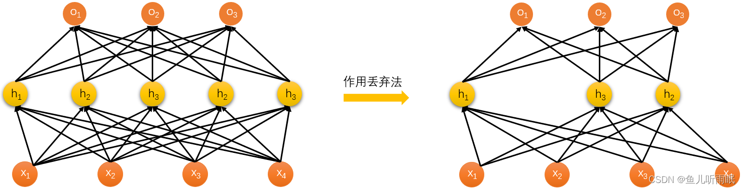
丢弃法： 在层之间加入噪音。

1.2 无偏差的加入噪音

对 $\vec x$ 加入噪音得到 $\vec x'$ ，我们希望：
$E[\vec x']=\vec x$
丢弃法对每个元素进行如下扰动：
$x_i'=\begin{cases}0 \qquad \text{with probablity} p \\ \frac{x_i}{1-p}\quad \text{otherise}\end{cases}$

1.3 使用丢弃法

1.3.1 训练中

通常将丢弃法作用在隐藏全连接层的输出上，例如：
$\begin{aligned} \vec h &= \sigma(W_1 \vec x + \vec b_1) \\ \vec h'&=\mathop{dropout}(\vec h) \\ \vec o &= W_2 \vec h' + \vec b_2 \\ \vec y &= \mathop{softmax}(\vec o) \end{aligned}$ 假设我们对一个单隐藏层的网络使用丢弃法，隐藏层的部分元素可能会被变为0。

丢弃法

1.3.2 预测中

正则项只在训练中使用：他们影响模型参数的更新。
在推理过程中，丢弃法直接返回输入：
$\vec h = \mathop{dropout} (\vec h)$
- 这样也可以保证确定性的输出。

1.4 总结

丢弃法将一些输出项随机置0来控制模型复杂度。
长作用在多层感知机的隐藏层输出上。
丢弃改了是控制模型复杂度的超参数。

二、代码实现

2.1 从零开始的实现

2.1.1 Dropout

我们实现dropout_layer函数，该函数以dropout的概率丢弃张量输入X中的元素。

import torch
from torch import nn
from d2l import torch as d2l

def dropout_layer(X, dropout):
    assert 0 <= dropout <= 1
    if dropout == 1:
        return torch.zeros_like(X)
    if dropout == 0:
        return X
    mask = (torch.randn(X.shape) > dropout).float()
    return mask * X / (1.0 - dropout)

上述代码中，torch.randn(X.shape)生成一个形状等同于X的在0到1之间的均匀随机分布。
我们可以来测试一下dropout函数：

# 测试dropout_layer函数
X = torch.arange(16, dtype=torch.float32).reshape((2, 8))
print(X)
print(dropout_layer(X, 0.))
print(dropout_layer(X, 0.5))
print(dropout_layer(X, 1.))

2.1.2 定义模型

我们定义一个具有两个隐藏层的多层感知机，每个隐藏层包含256个单元。

# 定义具有两个隐藏层的多层感知机
num_inputs, num_outputs, num_hiddens1, num_hiddens2 = 784, 10, 256, 256

dropout1, dropout2 = 0.2, 0.5

class Net(nn.Module):
    def __init__(self, num_inputs, num_outputs,
                 num_hiddens1, num_hiddens2, is_training = True):
        super(Net, self).__init__()
        self.num_inputs = num_inputs
        self.training = is_training
        self.lin1 = nn.Linear(num_inputs, num_hiddens1)
        self.lin2 = nn.Linear(num_hiddens1, num_hiddens2)
        self.lin3 = nn.Linear(num_hiddens2, num_outputs)
        self.relu = nn.ReLU()

    def forward(self, X):
        H1 = self.relu(self.lin1(X.reshape((-1, self.num_inputs))))
        if self.training == True:
            H1 = dropout_layer(H1, dropout1)
        H2 = self.relu(self.lin2(H1))
        if self.training == True:
            H2 = dropout_layer(H2, dropout2)
        out = self.lin3(H2)
        return out

2.1.3 训练和测试

# 训练和测试
num_epochs, lr, batch_size = 10, 0.5, 256
loss = nn.CrossEntropyLoss(reduction='none')
train_iter, test_iter = d2l.load_data_fashion_mnist(batch_size)
trainer = torch.optim.SGD(net.parameters(), lr=lr)
d2l.train_ch3(net, train_iter, test_iter, loss, num_epochs, trainer)

运行结果如下图所示：
实现1

2.2 简洁实现

2.2.1 定义模型与Dropout

# 简洁实现
net_concise = nn.Sequential(nn.Flatten(), nn.Linear(784, 256), nn.ReLU(),
                            nn.Dropout(dropout1), nn.Linear(256, 256), nn.ReLU(),
                            nn.Dropout(dropout2), nn.Linear(256, 10))

# 简洁实现 初始化权重
def init_weights(m):
    if type(m) == nn.Linear:
        nn.init.normal_(m.weight, std=0)

net.apply(init_weights)

2.2.2 训练和测试

trainer = torch.optim.SGD(net_concise.parameters(), lr)
d2l.train_ch3(net_concise, train_iter, test_iter, loss, num_epochs, trainer)

运行结果如下图所示：
实现2
下一篇：【动手学深度学习v2李沐】学习笔记09：数值稳定性、模型初始化、激活函数

【动手学深度学习v2李沐】学习笔记08：丢弃法

文章目录