使用线性回归推导函数实现线性回归

import numpy as np  # 导入科学技术框架

import matplotlib.pyplot as plt  # 导入画图工具

# 随机生成100个数据[0, 3)之间，rand是随机均匀分布[0, 1)
x = 3 * np.random.rand(100, 1)
# 生成y值
y = 3 + 4 * x + np.random.rand(100, 1)

# 整合x0和x1
# ones:创建任意维度和元素个数的数组，其元素值均为1，ones([100, 1])表示生成10行1列的二维数组
# c_:将切片对象沿第二轴（按列）转换为连接，与scala中的zip类似
x_b = np.c_[np.ones([100, 1]), x]
# print(x_b)

# 使用线性回归推导函数求解theta
# T:转置
# dot:矩阵乘或数组点积
# np.linalg.inv:逆矩阵
theta_best = np.linalg.inv(x_b.T.dot(x_b)).dot(x_b.T).dot(y)  # 线性回归推倒函数
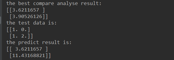
print("the best compare analyse result:\n{}".format(theta_best))

# 创建测试集x=0, 2
x_new = np.array([[0], [2]])
x_new_b = np.c_[(np.ones((2, 1))), x_new]
print("the test data is:\n{}".format(x_new_b))

# 进行预测：x=0时y应该等于3，x=2时y应该等于11
y_predict = x_new_b.dot(theta_best)
print("the predict result is:\n{}".format(y_predict))

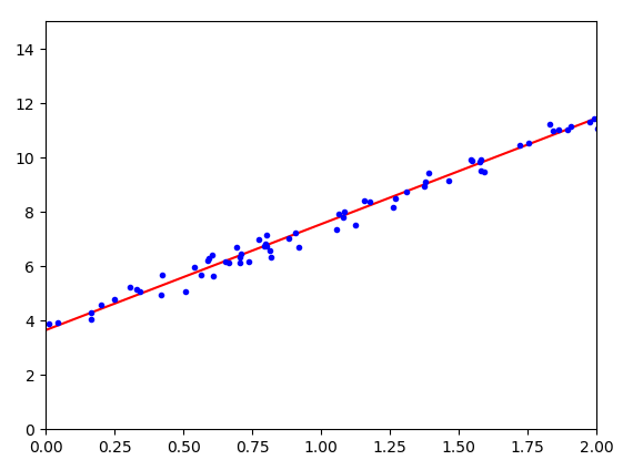
# 可视化展示
plt.plot(x_new, y_predict, "r-")  # 预测的线性回归直线
plt.plot(x, y, "b.")  # 生成的数据打点
plt.axis([0, 2, 0, 15])  # x,y轴设定，x:0~2,y:0~15
plt.show()  # 显示

结果：

 

可视化：