一、预测评价指标
分类问题的评价指标是准确率,回归算法的评价指标是MSE,RMSE,MAE。测试数据集中的点,距离模型的平均距离越小,该模型越精确。使用平均距离,而不是所有测试样本的距离和,因为受样本数量影响。假设如下:

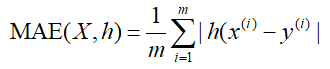
1、MAE----平均绝对误差损失
平均绝对误差,观测值与真实值的误差绝对值的平均值。
范围[0,+∞),当预测值与真实值完全吻合时等于0,即完美模型;误差越来大,值越大。
MAE 的曲线呈 V 字型,连续但在 y-f(x)=0 处不可导,计算机求解导数比较困难。而且 MAE 大部分情况下梯度都是相等的,这意味着即使对于小的损失值,其梯度也是大的。这不利于函数的收敛和模型的学习。
MAE 相比 MSE 有个优点就是 MAE 对离群点不那么敏感,更有包容性。因为 MAE 计算的是误差 y-f(x) 的绝对值,无论是 y-f(x)>1 还是 y-f(x)<1,没有平方项的作用,惩罚力度都是一样的,所占权重一样。

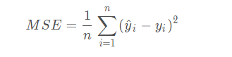
2、MSE----均方差损失
MSE是真实值与预测值的差值的平方然后求和平均。
范围[0,+∞),当预测值与真实值完全相同时为0,误差越大,该值越大。
MSE 曲线的特点是光滑连续、可导,便于使用梯度下降算法,是比较常用的一种损失函数。而且,MSE 随着误差的减小,梯度也在减小,这有利于函数的收敛,即使固定学习因子,函数也能较快取得最小值。
平方误差有个特性,就是当 yi 与 f(xi) 的差值大于 1 时,会增大其误差;当 yi 与 f(xi) 的差值小于 1 时,会减小其误差。这是由平方的特性决定的。
也就是说, MSE 会对误差较大(>1)的情况给予更大的惩罚,对误差较小(<1)的情况给予更小的惩罚。从训练的角度来看,模型会更加偏向于惩罚较大的点,赋予其更大的权重。
如果样本中存在离群点,MSE 会给离群点赋予更高的权重,但是却是以牺牲其他正常数据点的预测效果为代价,这最终会降低模型的整体性能。

3、RMSE----均方根误差
其实就是MSE加了个根号
范围[0,+∞),当预测值与真实值完全吻合时等于0,即完美模型;误差越大,该值越大。

4、差别
1、MAE---RMSE
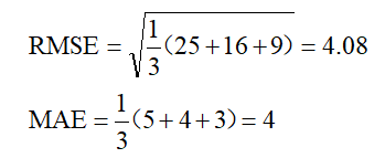
两个指标是用来描述预测值与真实值的误差情况。它们之间在的区别在于,RMSE先对偏差做了一次平方,如果误差的离散度高,也就是说,如果最大偏差值大的话,RMSE就放大了。
比如真实值是0,对于3次测量值分别是8,3,1,那么:
如果3次测量值分别是5,4,3,那么:
可以看出,两种情况下MAE相同,但是因为前一种情况下有更大的偏离值,所以RMSE就大的多了。

2、MAE---MSE
1、一般情况下,MSE收敛速度更快
2、MAE不易受到异常值影响
3、MAE损失与误差间为线性关系,而MSE与误差间则是平方关系,当误差越来越大,会使得MSE损失远远大于MAE损失,当MSE损失非常大时,对模型训练的影响也很大
4、MSE假设服从标准高分布,而MAE服从拉普拉斯分布而拉普拉斯分布本身就对异常值更具鲁棒性,当异常值出现时,拉普拉斯分布相比高斯分布受到的影响要小很多,因此以拉普拉斯分布假设的MAE在处理异常值是比高斯分布假设的MSE更加鲁棒
补充鲁棒性:
在统计学中,鲁棒性(Robustness)指的是某一估计量对数据中异常值的抵抗能力。简单来说,一个鲁棒的估计方法,能够在数据中包含离群值或异常点时仍能给出有效和稳健的结果。这种方法的优点在于,它们不会过度依赖于某些异常值而导致整个估计结果的失真。
在机器学习中,鲁棒性也是一个很重要的概念。当我们训练一个模型时,输入的数据中可能会包含一些异常值或噪声,这些异常值或噪声可能会导致模型的性能下降。一个鲁棒性强的模型能够在存在异常值或噪声的情况下依然有较好的性能表现。
通常情况下,鲁棒性的提高往往会以一些代价为代价,例如准确性的下降或计算成本的增加。因此,我们需要在鲁棒性和其他指标之间进行权衡,选择最适合当前任务的评估指标和模型。
二、三种梯度下降的结合
1、批量--MSE
import numpy as np
import matplotlib.pyplot as plt
from sklearn.datasets import load_iris
from sklearn.model_selection import train_test_split
# 加载数据集
iris = load_iris()
X = iris.data[:, 2] # 取花瓣长度特征
y = iris.data[:, 3]
# 数据标准化
X = (X - np.mean(X)) / np.std(X)
# 划分训练集和测试集
'''
这行代码使用了Scikit-learn库中的train_test_split函数,将原始数据集X和y划分成训练集和测试集。
其中,test_size=0.2表示测试集占总数据集的20%,即训练集占总数据集的80%;
random_state=42是为了保证每次随机划分数据集时都相同,方便后续的复现和比较。
划分后的数据集变量分别为X_train、X_test、y_train、y_test。
'''
X_train, X_test, y_train, y_test = train_test_split(X, y, test_size=0.2, random_state=42)
# 构建模型
theta = np.zeros(2) # 参数初始化
alpha = 0.01 # 学习率
iters = 1000 # 迭代次数
m_train = len(X_train) # 训练集样本数量
m_test = len(X_test) # 测试集样本数量
# 批量梯度下降算法
def bgd(X, y, theta, alpha, iters):
J_history = [] # 记录代价函数的值
for i in range(iters):
h = np.dot(X, theta) # 预测值
error = h - y # 误差
cost = 1 / (2 * m_train) * np.dot(error.T, error) # 计算代价函数
J_history.append(cost)
theta = theta - (alpha / m_train) * np.dot(X.T, error) # 更新参数
return theta, J_history
# 训练模型
X_train = np.c_[np.ones(m_train), X_train] # 增加一列全为1的特征
theta, J_history = bgd(X_train, y_train, theta, alpha, iters)
print("theta: ", theta)
# 在测试集上评估模型
X_test = np.c_[np.ones(m_test), X_test] # 增加一列全为1的特征
y_pred = np.dot(X_test, theta)
'''
这行代码是用来计算模型的均方误差(Mean Squared Error,MSE)的。
具体来说,它计算了模型在测试集上的预测值和实际值之差的平方的均值。MSE 越小,说明模型在测试集上的拟合效果越好。
其中,y_pred 是模型在测试集上的预测值,y_test 是测试集上的实际值。
用 (y_pred - y_test) ** 2 计算预测值和实际值之差的平方,然后再用 np.mean() 计算平均值,就得到了模型的 MSE。
'''
mse = np.mean((y_pred - y_test) ** 2)
print("MSE on test set: ", mse)
# 可视化
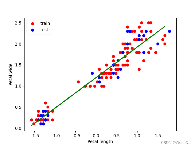
plt.scatter(X_train[:, 1], y_train, color='r')
plt.scatter(X_test[:, 1], y_test, color='b')
plt.plot(X_train[:, 1], np.dot(X_train, theta), color='g')
plt.xlabel('Petal length')
plt.ylabel('Petal wide')
plt.show()
# 绘制代价函数随迭代次数变化的曲线
plt.plot(np.arange(iters), J_history)
plt.xlabel('Iterations')
plt.ylabel('Cost')
plt.show()


2、批量--RMSE
import numpy as np
import matplotlib.pyplot as plt
from sklearn.datasets import load_iris
from sklearn.model_selection import train_test_split
from sklearn.metrics import mean_squared_error

# 加载数据集
iris = load_iris()
X = iris.data[:, 2]  # 取花瓣长度特征
y = iris.data[:, 3]

# 数据标准化
X = (X - np.mean(X)) / np.std(X)

# 划分训练集和测试集
X_train, X_test, y_train, y_test = train_test_split(X, y, test_size=0.2, random_state=42)

# 构建模型
theta = np.zeros(2)  # 参数初始化
alpha = 0.01  # 学习率
iters = 1000  # 迭代次数
m_train = len(X_train)  # 训练集样本数量
m_test = len(X_test)  # 测试集样本数量

# 批量梯度下降算法
def bgd(X, y, theta, alpha, iters):
    J_history = []  # 记录代价函数的值
    for i in range(iters):
        h = np.dot(X, theta)  # 预测值
        error = h - y  # 误差
        cost = 1 / (2 * m_train) * np.dot(error.T, error)  # 计算代价函数
        J_history.append(cost)
        theta = theta - (alpha / m_train) * np.dot(X.T, error)  # 更新参数
    return theta, J_history

# 训练模型
X_train = np.c_[np.ones(m_train), X_train]  # 增加一列全为1的特征
theta, J_history = bgd(X_train, y_train, theta, alpha, iters)
print("theta: ", theta)

# 在测试集上评估模型
X_test = np.c_[np.ones(m_test), X_test]  # 增加一列全为1的特征
y_pred = np.dot(X_test, theta)
rmse = np.sqrt(mean_squared_error(y_test, y_pred))
'''
mean_squared_error(y_test, y_pred):该函数接受两个参数,即真实值 y_test 和预测值 y_pred。
它计算它们之间的均方误差(MSE),即两个数组中对应元素差值的平方的平均值。
np.sqrt():该函数用于求算术平方根,即对 MSE 取平方根,得到 RMSE。
'''
print("RMSE on test set: ", rmse)

# 可视化
plt.scatter(X_train[:, 1], y_train, label='train', color='blue')
plt.scatter(X_test[:, 1], y_test, label='test', color='red')
plt.plot(X_train[:, 1], np.dot(X_train, theta), color='green')
plt.xlabel('Petal length')
plt.ylabel('Petal wide')
plt.legend()
plt.show()

# 绘制代价函数随迭代次数变化的曲线
plt.plot(np.arange(iters), J_history)
plt.xlabel('Iterations')
plt.ylabel('Cost')
plt.show()


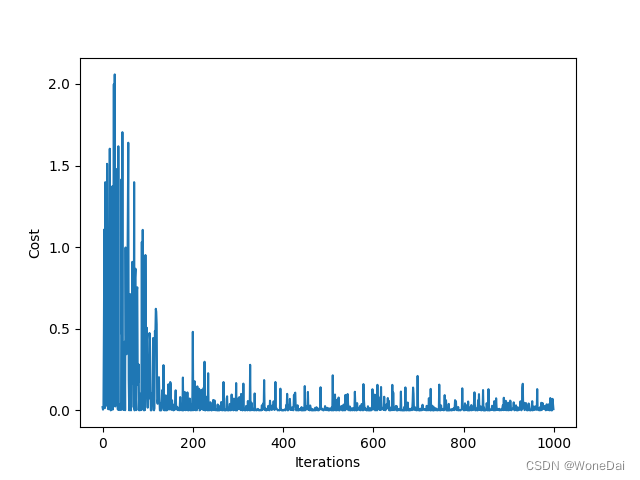
3、小批量--MSE
import numpy as np
import matplotlib.pyplot as plt
from sklearn.datasets import load_iris
from sklearn.model_selection import train_test_split
from sklearn.metrics import mean_squared_error

# 加载数据集
iris = load_iris()
X = iris.data[:, 2]  # 取花瓣长度特征
y = iris.data[:, 3]

# 数据标准化
X = (X - np.mean(X)) / np.std(X)

# 划分训练集和测试集
X_train, X_test, y_train, y_test = train_test_split(X, y, test_size=0.2, random_state=42)

# 构建模型
theta = np.zeros(2)  # 参数初始化
alpha = 0.01  # 学习率
iters = 1000  # 迭代次数
batch_size = 16  # 小批量大小
m_train = len(X_train)  # 训练集样本数量
m_test = len(X_test)  # 测试集样本数量

# 小批量梯度下降算法
def mini_batch_gd(X, y, theta, alpha, iters, batch_size):
    J_history = []  # 记录代价函数的值
    for i in range(iters):
        # 从训练集中随机选择一个小批量
        idx = np.random.choice(m_train, batch_size, replace=False)
        X_batch = X[idx]
        y_batch = y[idx]
        h = np.dot(X_batch, theta)  # 预测值
        error = h - y_batch  # 误差
        cost = mean_squared_error(y_batch, h)  # 计算代价函数(MSE)
        # cost = 1 / (2 * batch_size) * np.dot(error.T, error)  # 计算代价函数
        J_history.append(cost)
        theta = theta - (alpha / batch_size) * np.dot(X_batch.T, error)  # 更新参数
    return theta, J_history

# 训练模型
X_train = np.c_[np.ones(m_train), X_train]  # 增加一列全为1的特征
theta, J_history = mini_batch_gd(X_train, y_train, theta, alpha, iters, batch_size)
print("theta: ", theta)

# 在测试集上评估模型
X_test = np.c_[np.ones(m_test), X_test]  # 增加一列全为1的特征
y_pred = np.dot(X_test, theta)
mse = mean_squared_error(y_test, y_pred)  # MSE
print("MSE on test set: ", mse)

# 可视化
plt.scatter(X_train[:, 1], y_train, color='r', label='Training set')
plt.scatter(X_test[:, 1], y_test, color='b', label='Testing set')
plt.plot(X_train[:, 1], np.dot(X_train, theta), color='g', label='Regression line')
plt.xlabel('Petal length')
plt.ylabel('Petal wide')
plt.legend()
plt.show()

# 绘制代价函数随迭代次数变化的曲线
plt.plot(np.arange(iters), J_history)
plt.xlabel('Iterations')
plt.ylabel('Cost')
plt.show()


4、小批量--RMSE
import numpy as np
import matplotlib.pyplot as plt
from sklearn.datasets import load_iris
from sklearn.model_selection import train_test_split
from sklearn.metrics import mean_squared_error

# 加载数据集
iris = load_iris()
X = iris.data[:, 2]  # 取花瓣长度特征
y = iris.data[:, 3]

# 数据标准化
X = (X - np.mean(X)) / np.std(X)

# 划分训练集和测试集
X_train, X_test, y_train, y_test = train_test_split(X, y, test_size=0.2, random_state=42)

# 构建模型
theta = np.zeros(2)  # 参数初始化
alpha = 0.01  # 学习率
iters = 1000  # 迭代次数
batch_size = 16  # 小批量大小
m_train = len(X_train)  # 训练集样本数量
m_test = len(X_test)  # 测试集样本数量

# 小批量梯度下降算法
def mini_batch_gd(X, y, theta, alpha, iters, batch_size):
    J_history = []  # 记录代价函数的值
    for i in range(iters):
        # 从训练集中随机选择一个小批量
        idx = np.random.choice(m_train, batch_size, replace=False)
        X_batch = X[idx]
        y_batch = y[idx]
        h = np.dot(X_batch, theta)  # 预测值
        error = h - y_batch  # 误差
        cost = 1 / (2 * batch_size) * np.dot(error.T, error)  # 计算代价函数
        J_history.append(cost)
        theta = theta - (alpha / batch_size) * np.dot(X_batch.T, error)  # 更新参数
    return theta, J_history

# 训练模型
X_train = np.c_[np.ones(m_train), X_train]  # 增加一列全为1的特征
theta, J_history = mini_batch_gd(X_train, y_train, theta, alpha, iters, batch_size)
print("theta: ", theta)

# 在测试集上评估模型
X_test = np.c_[np.ones(m_test), X_test]  # 增加一列全为1的特征
y_pred = np.dot(X_test, theta)
rmse = np.sqrt(mean_squared_error(y_test, y_pred))
print("RMSE on test set: ", rmse)

# 可视化
plt.scatter(X_train[:, 1], y_train, color='r', label='Training set')
plt.scatter(X_test[:, 1], y_test, color='b', label='Testing set')
plt.plot(X_train[:, 1], np.dot(X_train, theta), color='g', label='Regression line')
plt.xlabel('Petal length')
plt.ylabel('Petal wide')
plt.legend()
plt.show()

# 绘制代价函数随迭代次数变化的曲线
plt.plot(np.arange(iters), J_history)
plt.xlabel('Iterations')
plt.ylabel('Cost (RMSE)')
plt.show()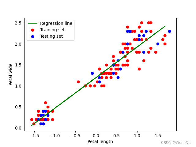


5、随机--MSE
import numpy as np
import matplotlib.pyplot as plt
from sklearn.datasets import load_iris
from sklearn.model_selection import train_test_split

# 加载数据集
iris = load_iris()
X = iris.data[:, 2]  # 取花瓣长度特征
y = iris.data[:, 3]

# 数据标准化
X = (X - np.mean(X)) / np.std(X)

# 划分训练集和测试集
'''
在sklearn的train_test_split函数中,可以通过设置random_state参数来控制随机划分的结果可复现性。
这个参数可以是一个整数,也可以是一个随机数生成器的实例。
当random_state参数的值固定时,每次运行train_test_split函数都会得到相同的随机划分结果,这样就保证了实验的可重复性。
在实际应用中,通常将random_state设置为一个固定的整数,比如42。
'''
X_train, X_test, y_train, y_test = train_test_split(X, y, test_size=0.2, random_state=22)

# 构建模型
theta = np.zeros(2)  # 参数初始化
alpha = 0.01  # 学习率
iters = 1000  # 迭代次数
m = len(X_train)  # 训练集样本数量

# 随机梯度下降算法
def sgd(X, y, theta, alpha, iters):
    J_history = []  # 记录代价函数的值
    for i in range(iters):
        # 随机选择一个样本
        random_index = np.random.randint(0, m)
        xi = X[random_index]
        yi = y[random_index]
        # 预测值
        h = np.dot(xi, theta)
        error = h - yi  # 误差
        cost = 1 / 2 * (error ** 2)  # 计算代价函数
        J_history.append(cost)
        # 更新参数
        theta = theta - alpha * error * xi.T
    return theta, J_history

# 训练模型
X_train = np.c_[np.ones(m), X_train]  # 增加一列全为1的特征
theta, J_history = sgd(X_train, y_train, theta, alpha, iters)
print("theta: ", theta)

# 可视化
plt.scatter(X_train[:, 1], y_train, color='r', label='Training set')
plt.scatter(X_test, y_test, color='b',label='Testing set')
plt.plot(X_train[:, 1], np.dot(X_train, theta), color='g', label='Regression line')
plt.xlabel('Petal length')
plt.ylabel('Petal wide')
plt.legend()
plt.show()

# 绘制代价函数随迭代次数变化的曲线
plt.plot(np.arange(iters), J_history)
plt.xlabel('Iterations')
plt.ylabel('Cost')
plt.show()

# 计算测试集MSE
X_test = np.c_[np.ones(len(X_test)), X_test]  # 增加一列全为1的特征
y_test_pred = np.dot(X_test, theta)
mse_test = np.mean((y_test_pred - y_test) ** 2)
print("MSE on test set: ", mse_test)


6、随机--RMSE
import numpy as np
import matplotlib.pyplot as plt
from sklearn.datasets import load_iris
from sklearn.model_selection import train_test_split

# 加载数据集
iris = load_iris()
X = iris.data[:, 2]  # 取花瓣长度特征
y = iris.data[:, 3]

# 数据标准化
X = (X - np.mean(X)) / np.std(X)

# 划分训练集和测试集
X_train, X_test, y_train, y_test = train_test_split(X, y, test_size=0.2, random_state=22)

# 构建模型
theta = np.zeros(2)  # 参数初始化
alpha = 0.01  # 学习率
iters = 1000  # 迭代次数
m = len(X_train)  # 训练集样本数量

# 随机梯度下降算法
def sgd(X, y, theta, alpha, iters):
    J_history = []  # 记录代价函数的值
    for i in range(iters):
        # 随机选择一个样本
        random_index = np.random.randint(0, m)
        xi = X[random_index]
        yi = y[random_index]
        # 预测值
        h = np.dot(xi, theta)
        error = h - yi  # 误差
        cost = 1 / 2 * (error ** 2)  # 计算代价函数
        J_history.append(cost)
        # 更新参数
        theta = theta - alpha * error * xi.T
    return theta, J_history

# 训练模型
X_train = np.c_[np.ones(m), X_train]  # 增加一列全为1的特征
theta, J_history = sgd(X_train, y_train, theta, alpha, iters)
print("theta: ", theta)

# 可视化
plt.scatter(X_train[:, 1], y_train, color='r', label='Training set')
plt.scatter(X_test, y_test, color='b', label='Testing set')
plt.plot(X_train[:, 1], np.dot(X_train, theta), color='g', label='Regression line')
plt.xlabel('Petal length')
plt.ylabel('Petal wide')
plt.legend()
plt.show()

# 绘制代价函数随迭代次数变化的曲线
plt.plot(np.arange(iters), J_history)
plt.xlabel('Iterations')
plt.ylabel('Cost')
plt.show()

# 计算测试集RMSE
X_test = np.c_[np.ones(len(X_test)), X_test]  # 增加一列全为1的特征
y_test_pred = np.dot(X_test, theta)
mse_test = np.mean((y_test_pred - y_test) ** 2)
rmse_test = np.sqrt(mse_test)
print("RMSE on test set: ", rmse_test)


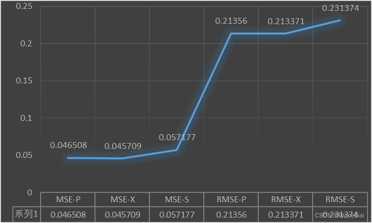
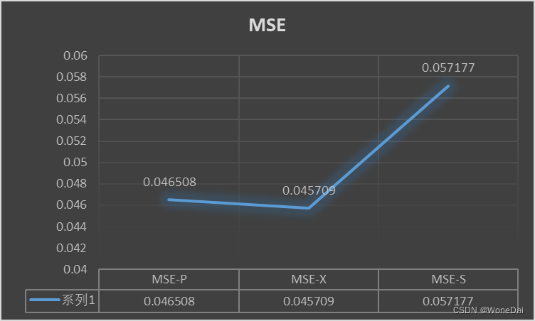
三、结果观察

参考内容来源:
(8条消息) MSE(均方误差)函数和RMSE函数_rmse和mse_痴迷、淡然~的博客-CSDN博客