《机器学习公式推导与代码实现》学习笔记,记录一下自己的学习过程,详细的内容请大家购买作者的书籍查阅。
集成学习:对比与调参
虽然现在深度学习大行其道,但以XGBoost、LightGBM、CatBoost为代表的Boosting算法仍有其广泛的用武之地。抛开深度学习适用的文本、图像、语音和视频等非结构化数据应用,对于训练样本较少的结构化数据领域,Boosting算法仍然是第一选择。
1 三大Boosting算法对比
XGBoost、LightGBM和CatBoost都是目前经典的SOTA(state of the art)Boosting算法,这三个模型都是以决策树为支撑的集成学习框架,其中XGBoost是对原始版本GBDT算法的改进,而LightGBM和CatBoost在XGBoost基础上做了进一步的优化,在精度和速度上各有所长。
三大Boosting算法主要有两个方面的区别:
第一,模型树的构造方式有所不同,XGBoost使用按层生长(level-wise)的决策树构建策略,LightGBM则使用按叶子生长(leaf-wise)的构建策略,而CatBoost使用对称树结构(oblivious-tree),其决策树都是完全二叉树。
第二,对于类别特征的处理有较大区别,XGBoost本身不具备自动处理类别特征的能力,对于数据中的类别特征,需要我们手动处理变换成数值后才能输入到模型中;LightGBM中则需要指定类别特征名称,算法会自动对齐进行处理;CatBoost以处理类别特征而闻名,通过目标变量统计等特征编码方式也能实现高效处理类别特征。
1.1 数据预处理
下面以 Kaggle 2015年的flights数据集为例,分别用XGBoost、LightGBM和CatBoost模型进行实验:
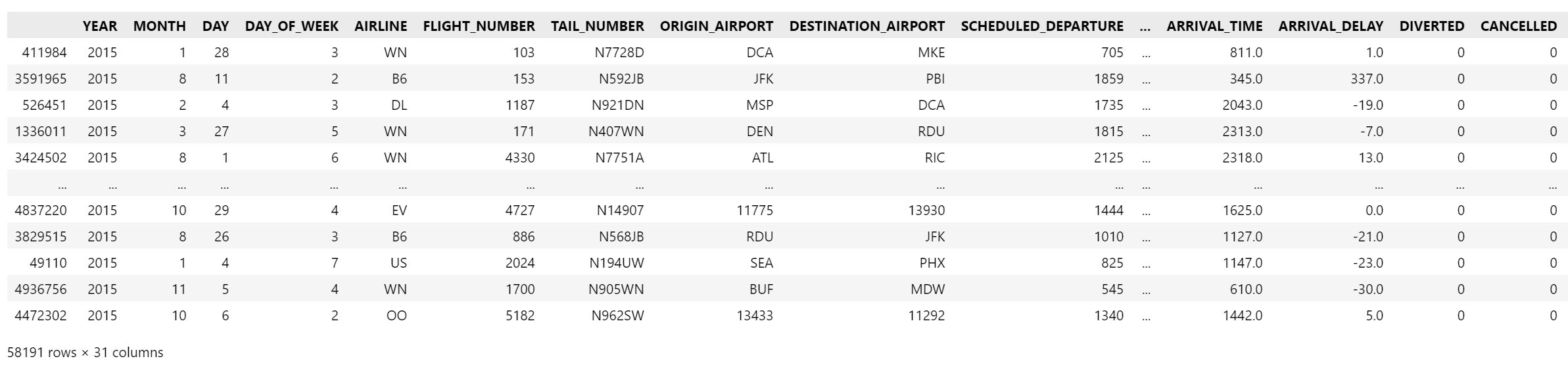
flights数据集
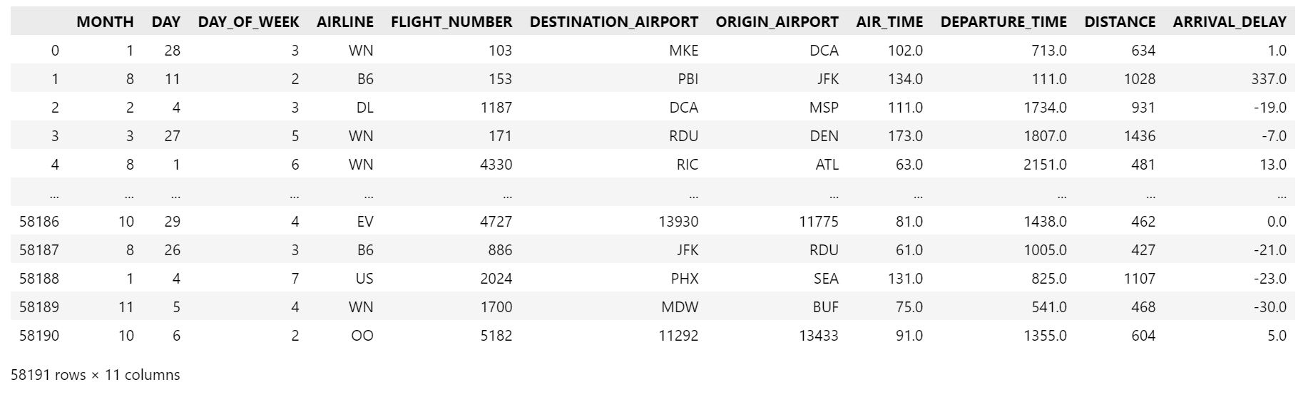
该数据集共有500多万条航班记录数据,特征有31个。我们采取抽样的方式从原始数据集中抽取1%的数据,并筛选11个特征用作演示,经过预处理后重新构建训练集,目标是构建对航班是否延误的二分类模型。
import pandas as pd
from sklearn.model_selection import train_test_split
flights = pd.read_csv('flights.csv')
flights = flights.sample(frac=0.01, random_state=10) # 数据集抽样1%
flights
flights = flights[["MONTH","DAY","DAY_OF_WEEK","AIRLINE","FLIGHT_NUMBER","DESTINATION_AIRPORT",
                 "ORIGIN_AIRPORT","AIR_TIME", "DEPARTURE_TIME","DISTANCE","ARRIVAL_DELAY"]] # 选11个特征
flights= flights.reset_index(drop=True)
flights
flights["ARRIVAL_DELAY"] = (flights["ARRIVAL_DELAY"]>10)*1 # 延误超过10分钟看作是延误,bool类型转换为int类型
flights["ARRIVAL_DELAY"].unique()
array([0, 1], dtype=int32)
cols = ["AIRLINE","FLIGHT_NUMBER","DESTINATION_AIRPORT","ORIGIN_AIRPORT"] # 类别特征
for col in cols:
    print(len(flights[col].unique()))
14
6163
633
644
for item in cols:
    flights[item] = flights[item].astype("category").cat.codes

X_train, X_test, y_train, y_test = train_test_split(flights.drop(["ARRIVAL_DELAY"], axis=1), flights["ARRIVAL_DELAY"], random_state=10, test_size=0.3) # 划分数据集
1.2 XGBoost在flights数据集上的测试
from sklearn.metrics import roc_auc_score
import xgboost as xgb
import time

# 设置模型参数
params = {


    'booster': 'gbtree', # 基于树
    'objective': 'binary:logistic',
    'gamma': 0.1, # 剪枝中用到的最小损失下降值
    'max_depth': 8,
    'lambda': 2,
    'subsample': 0.7, # 表示用于训练的样本比例
    'colsample_bytree': 0.7, # 表示用于训练的特征比例
    'min_child_weight': 3, # 一个叶子节点的最小权重
    'eta': 0.001,# 学习速率
    'seed': 1000,
    'nthread': 4, # 线程数量,用于并行计算
}

# 训练
t0 = time.time()
num_rounds = 500 # 表示训练轮数,即树的个数
dtrain = xgb.DMatrix(X_train, y_train)
model_xgb = xgb.train(params, dtrain, num_rounds)
print('training spend {} seconds'.format(time.time()-t0))

# 测试
t1 = time.time()
dtest = xgb.DMatrix(X_test)
y_pred = model_xgb.predict(dtest)
print('testing spend {} seconds'.format(time.time()-t1))
y_pred_train = model_xgb.predict(dtrain)
print(f"训练集auc:{

      roc_auc_score(y_train, y_pred_train)}")
print(f"测试集auc:{

      roc_auc_score(y_test, y_pred)}")
training spend 6.46193265914917 seconds
testing spend 0.057062625885009766 seconds
训练集auc:0.752049936354563
测试集auc:0.6965194979943091
1.3 LightGBM在flights数据集上的测试
import lightgbm as lgb
d_train = lgb.Dataset(X_train, label=y_train)

# 设置模型参数
params = {


    "max_depth": 5,
    "learning_rate" : 0.05,
    "num_leaves": 500,
    "n_estimators": 300
}

cate_features_name = ["MONTH","DAY","DAY_OF_WEEK","AIRLINE","DESTINATION_AIRPORT", "ORIGIN_AIRPORT"] # 类别特征

t0 = time.time()
model_lgb = lgb.train(params, d_train, categorical_feature = cate_features_name)
print('training spend {} seconds'.format(time.time()-t0))
t1 = time.time()

y_pred = model_lgb.predict(X_test)
print('testing spend {} seconds'.format(time.time()-t1))
y_pred_train = model_lgb.predict(X_train)
print(f"训练集auc:{

      roc_auc_score(y_train, y_pred_train)}")
print(f"测试集auc:{

      roc_auc_score(y_test, y_pred)}")
training spend 0.43550848960876465 seconds
testing spend 0.0230252742767334 seconds
训练集auc:0.8867447004324996
测试集auc:0.7033506245405025
1.2 CatBoost在flights数据集上的测试
import catboost as cb
cat_features_index = [0,1,2,3,4,5,6]

t0 = time.time()
model_cb = cb.CatBoostClassifier(eval_metric="AUC", one_hot_max_size=50, depth=6, iterations=300, l2_leaf_reg=1, learning_rate=0.1)
model_cb.fit(X_train,y_train, cat_features= cat_features_index)
print('training spend {} seconds'.format(time.time()-t0))

t1 = time.time()
y_pred = model_cb.predict(X_test)
print('testing spend {} seconds'.format(time.time()-t1))
y_pred_train = model_cb.predict(X_train)
print(f"训练集auc:{

      roc_auc_score(y_train, y_pred_train)}")
print(f"测试集auc:{

      roc_auc_score(y_test, y_pred)}")
training spend 20.633496284484863 seconds
testing spend 0.03611636161804199 seconds
训练集auc:0.5670692017560355
测试集auc:0.5473357824098838
由上面的实验结果可以看出在没有做进一步数据特征工程和超参数调优的情况下,在该数据集上,LightGBM无论是精度上还是速度上都要优于XGBoost和CatBoost,CatBoost的表现最差。
2 常用超参数调优方法
我们将不经过模型训练得到的参数叫做超参数(hyperparameter),机器学习中常用的调参方法包括网格搜索法(grid search)、随机搜索法(random search)和贝叶斯优化(bayesian optimization)。
2.1 网格搜索法
网格搜索法是一种常用的超参数调优方法,常用于优化三个或者更少数量的超参数,本质上是一种穷举法。对于每个超参数,使用者选择一个较小的有限集去搜索,然后将这些超参数经过笛卡尔乘积得到若干组超参数。网格搜索使用每组超参数训练模型,挑选验证集误差最小的超参数作为最优化超参数。
sklearn通过model_selection模块下的GridSearchCV来实现网格搜索调参,并且这个调参过程是加了交叉验证的。下面展示XGBoost的网格搜索示例:
# 基于XGBoost的GridSearch搜索范例
from sklearn.model_selection import GridSearchCV

model = xgb.XGBClassifier()

# 待搜索的参数列表实例
params_lst = {


    'max_depth': [3,5,7],
    'min_child_weight': [1,3,6],
    'n_estimators': [100,200,300],
    'learning_rate': [0.01, 0.05, 0.1]
}

# verbose:表示日志输出的详细程度
# n_jobs:表示并行计算的数量,即同时运行的任务数,-1 表示使用所有可用的 CPU 进行并行计算
t0 = time.time()
grid_search = GridSearchCV(model, param_grid=params_lst, cv=3, verbose=10, n_jobs=-1)
grid_search.fit(X_train, y_train)
print('gridsearch for xgb spend', time.time()-t0, 'seconds.')
print(grid_search.best_params_)
gridsearch for xgb spend 67.24716424942017 seconds.
{

    'learning_rate': 0.1, 'max_depth': 5, 'min_child_weight': 6, 'n_estimators': 300}
2.2 随机搜索
随即搜索是在指定超参数范围内或者分布上随即搜寻最优超参数。相较于网格搜索方法,给定超参数分布,并不是所有超参数都要尝试,而是会从给定分布中抽样固定数量的参数,实际仅对这些抽样到的超参数进行实验。
sklearn通过model_selection模块下的RandomizedSearchCV方法进行随即搜索。
# 基于XGBoost的RandomizedSearch搜索范例
from sklearn.model_selection import RandomizedSearchCV # 通过 n_iter 进行手动设置或是自动根据参数空间大小确定采样次数

model = xgb.XGBClassifier()

# 待搜索的参数列表实例
params_lst = {


    'max_depth': [3,5,7],
    'min_child_weight': [1,3,6],
    'n_estimators': [100,200,300],
    'learning_rate': [0.01, 0.05, 0.1]
}

t0 = time.time()
random_search = RandomizedSearchCV(model, params_lst, random_state=0)
random_search.fit(X_train, y_train)
print(random_search.best_params_)
print('randomsearch for xgb spend', time.time()-t0, 'seconds.')
{

    'n_estimators': 300, 'min_child_weight': 6, 'max_depth': 5, 'learning_rate': 0.1}
randomsearch for xgb spend 60.41917014122009 seconds.
2.3 贝叶斯调参
贝叶斯调参(Bayesian Optimization)是一种基于贝叶斯定理的超参数优化方法,主要用于优化黑盒函数。相对于传统的网格搜索或随机搜索,贝叶斯调参基于样本观测的不确定性建立模型,通过贝叶斯公式计算后验分布,从中选择期望相对较高的超参数进行优化。
贝叶斯调参的关键思想是利用样本观测不断地更新模型的先验(前提假设),并在已知前提基础上预测下一个实验的结果。通过预测的结果,更新模型的后验分布,即已知样本后,超参数分布的概率密度函数。在超参数概率密度函数的统计学指标(比如期望和方差)的基础上,生成下一组超参数值,直到达到最优结果为止。在整个过程中,下一组待测试的超参数都是在当前已有数据的基础上,反向计算已有样本的超参数概率分布,并根据超参数的期望值(或模式)来进行搜索,在一定程度上使搜索更加“聪明”和高效。
在执行贝叶斯优化之前,我们需要基于XGBoost的交叉验证xgb.cv定义一个待优化的目标函数,获取xgb.cv交叉验证验证结果,并以测试集AUC为优化时的精度衡量指标。最后将定义好的目标优化函数和超参数搜索范围传入贝叶斯优化函数中,给定初始化点和迭代次数,即可执行贝叶斯优化。
# 定义相关参数
num_rounds = 3000

params = {


    'eta': 0.1,
    'silent': 1,
    'eval_metric': 'auc',
    'verbose_eval': True,
    'seed': 2023
}

# 定义目标优化函数
def xgb_evaluate(min_child_weight, colsample_bytree, max_depth, subsample, gamma,alpha):

    params['min_child_weight'] = int(min_child_weight)
    params['cosample_bytree'] = max(min(colsample_bytree, 1), 0)
    params['max_depth'] = int(max_depth)
    params['subsample'] = max(min(subsample, 1), 0)
    params['gamma'] = max(gamma, 0)
    params['alpha'] = max(alpha, 0)

    cv_result = xgb.cv(params, dtrain, num_boost_round=num_rounds, nfold=5, seed=2023, callbacks=[xgb.callback.EarlyStopping(rounds=50)])

    return cv_result['test-auc-mean'].values[-1]
# pip install bayesian-optimization
from bayes_opt import BayesianOptimization
#-*-coding:utf-8-*-

num_iter = 25
init_points = 5

t0 = time.time()
xgbBO = BayesianOptimization(xgb_evaluate, {


    'min_child_weight': (1, 20),
    'colsample_bytree': (0.1, 1),
    'max_depth': (5, 15),
    'subsample': (0.5, 1),
    'gamma': (0, 10),
    'alpha': (0, 10),
})
xgbBO.maximize(init_points=init_points, n_iter=num_iter)
print('bayesianSearch for xgb spend', time.time()-t0, 'seconds.')
|   iter    |  target   |   alpha   | colsam... |   gamma   | max_depth | min_ch... | subsample |
| 1         | 0.7193    | 7.155     | 0.5762    | 0.9578    | 9.488     | 13.18     | 0.9343    |
bayesianSearch for xgb spend 765.5525000095367 seconds.
可以看到,经过贝叶斯调参后的得到的参数使得xgboost在flights测试集上的auc值达到了0.72。