1. MobileNet v1网络

2. MobileNet v2网络

2.1 Inverted Residual

2.2 Linear Bottlenecks

2.3 MobileNet v2模型的网络结构

3.4 MobileNet v3模型的网络结构

扫描二维码关注公众号，回复： 15382331 查看本文章

4. 利用Pytorch实现MobileNet

4.1 MobileNet v1、v2

4.2 MobileNet v3

5. 训练结果

1. MobileNet v1网络

在传统的卷积神经网络中，模型参数都比较大，而且对算力的要求很高，很难在移动设备和嵌入式设备上运行，MobileNet实现了将深度学习网络在移动设备和嵌入式设备上运行。

MobileNet网络是Google团队在2017年提出的，是专注于移动端或者嵌入式设备中的轻量级CNN网络。相比传统CNN网络，在准确率小幅度降低的前提下大大减少了模型的参数和运算量。该网络有以下两个亮点：

Depthwise Convolution（DW卷积，大大减少了参数数量和运算量）

增加了控制卷积核个数的超参数 $\alpha$ 和控制输入图像大小的超参数 $\beta$

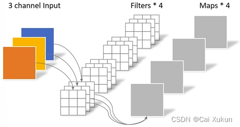
在传统的卷积操作中，卷积核的channel数等于输入特征矩阵的channel数，输出特征矩阵的channel数等于所使用卷积核的个数：

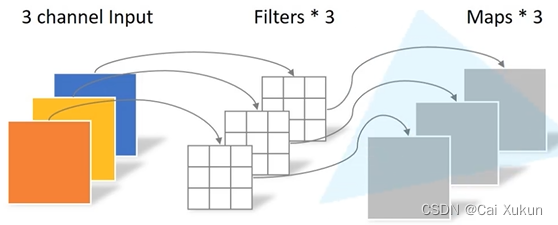
而对于DW卷积，卷积核的channel数为1，输入特征矩阵的channel数等于卷积核个数等于输出特征矩阵channel数：

Depthwise Separable Conv由DW卷积和PW卷积组成，PW卷积和传统卷积操作相似，只是卷积核大小均为1×1，理论上传统卷积的计算量是Depthwise Separable Conv操作的8到9倍。

2. MobileNet v2网络

在MobileNet的使用当中，DW卷积的卷积核参数大部分为0，这部分的卷积核没有起到作用，这个问题在MobileNet v2中有所改善，该网络有以下两个亮点：

Inverted Residual（倒残差结构）

Linear Bottlenecks

2.1 Inverted Residual

传统的残差结构是先用1×1的卷积核进行降维，然后通过3×3的卷积核进行卷积处理，最后采用1×1的卷积核进行升维，形成了一个两头大中间小的瓶颈结构；而倒残差结构首先利用1×1的卷积核进行升维，然后通过3×3的卷积核进行DW卷积，最后采用1×1的卷积核进行降维处理，和普通的残差结构正好相反。

在普通的残差结构中采用的是ReLU激活函数，而在倒残差结构中采用的则是ReLU6激活函数：

ReLU激活函数：输入值小于0时默认置0，输入值大于0则不进行操作

ReLU6激活函数：输入值小于0默认置0，输入值在0~6之间不进行操作，而输入值大于6时则置6，公式为

$y=ReLU6\left ( x \right )=min\left ( max\left ( x,0 \right ) ,6\right )$

2.2 Linear Bottlenecks

针对倒残差结构的最后一个卷积层，使用了线性的激活函数而非ReLU激活函数，原文作者进行了实验，内容是ReLU激活函数对低维特征信息会造成大量损失，对高维特征信息造成的损失很小，而倒残差结构是两边细中间粗的结构，输出是一个低维的特征向量，因此使用ReLU激活函数损失会比较大，所以使用线性的激活函数进行替代。

MobileNet v2的block块如下图所示：

要注意只有stride=1且输入特征矩阵与输出特征矩阵的shape相同时才有shortcut连接（即左面那种情况）。

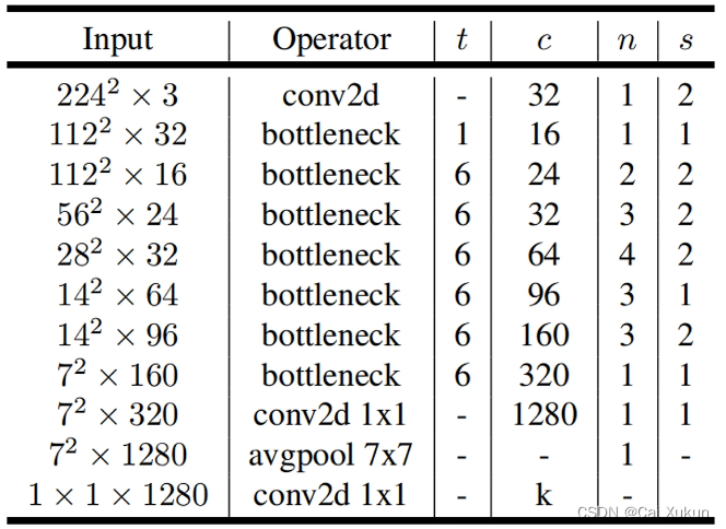
2.3 MobileNet v2模型的网络结构

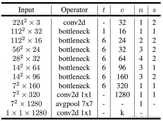
$t$ 为扩展因子，即将输入升为多少维；

$c$ 为输出特征矩阵深度；

$n$ 为bottleneck的重复次数；

$s$ 为第一层bottleneck的步长，其余层均为1。

3. MobileNet v3网络

MobileNet v3有以下三个改进点：

更新了Block（bneck，在倒残差结构上进行了简单的改动）

使用了NAS（Neural Architecture Search）搜索参数的技术

重新设计了一些耗时层的结构

对于Block的更新主要有亮点：加入了SE模块，更新了激活函数。结构图如下：

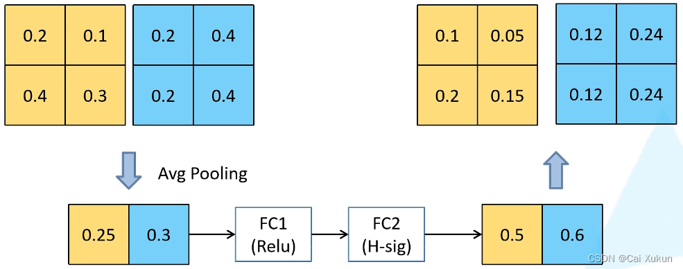
3.1 注意力机制

针对得到的输出矩阵的每个channel进行池化处理，得到一维向量的元素个数等于channel数；经过第一个全连接层，节点个数是channel个数的1/4，激活函数是ReLU；经过第二个全连接层，节点个数等于channel个数，激活函数是hard-sigmoid；最后输出的向量是对矩阵的每个channel分析出了权重关系，重要的channel会分配一个比较大的权重，原理图如下：

3.2 重新设计耗时层结构

减少第一个卷积层的卷积核个数，从32减到16，并且不会影响准确率；精简Last Stage，精简之前的模型如下：

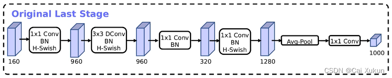
精简之后的模型：

3.3 重新设计激活函数

当时比较常用的激活函数是swish激活函数：

$swishx=x\cdot \sigma \left ( x \right )$

其中

$\sigma \left ( x \right )=\frac{1}{1+e^{-x}}$

这个激活函数的计算和求导很复杂；对于移动端的设备，为了加速都会进行量化操作，而swish激活函数对于量化操作很复杂。针对这两个问题，提出了h-swish激活函数：

$h-swish\left [ x \right ]=x\cdot \frac{ReLU6\left ( x+3 \right )}{6}$

式子中的后半部分是h-sigmoid激活函数。

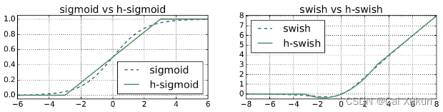
从图中可以看出，两种激活函数很相似，可以用h-swish替代swish使用，还可以简化量化操作。

3.4 MobileNet v3模型的网络结构

4. 利用Pytorch实现MobileNet

4.1 MobileNet v1、v2

在MobileNet v2网络当中，所有的卷积层基本都是卷积+BN+ReLU6激活函数组成，首先定义这个组合：

class ConvBNReLU(nn.Sequential):
    # 输入特征矩阵深度，输出特征矩阵深度，卷积核大小，步长，groups=1是普通卷积、=in_channel是DW卷积
    def __init__(self, in_channel, out_channel, kernel_size=3, stride=1, groups=1):
        # 填充参数
        padding = (kernel_size - 1) // 2
        super(ConvBNReLU, self).__init__(
            # 首先是卷积操作：输入特征矩阵深度，输出特征矩阵深度，卷积核大小，步长，填充参数，groups为默认值，不需要偏置
            nn.Conv2d(in_channel, out_channel, kernel_size, stride, padding, groups=groups, bias=False),
            # BN层，输入为卷积操作的输出
            nn.BatchNorm2d(out_channel),
            # 激活函数
            nn.ReLU6(inplace=True)
        )

倒残差结构：

# 倒残差结构
class InvertedResidual(nn.Module):
    # 输入特征矩阵深度，输出特征矩阵深度，步长，深度扩大多少倍
    def __init__(self, in_channel, out_channel, stride, expand_ratio):
        super(InvertedResidual, self).__init__()
        # 第一层卷积层，扩展深度
        hidden_channel = in_channel * expand_ratio
        # 定义一个布尔变量，步长为1且输入和输出特征矩阵相等时，采用捷径分支
        self.use_shortcut = stride == 1 and in_channel == out_channel

        # 层列表
        layers = []
        # t = 1时没有对输入特征矩阵进行扩充，此时不需要第一层卷积层
        if expand_ratio != 1:
            # 1x1 pointwise conv
            layers.append(ConvBNReLU(in_channel, hidden_channel, kernel_size=1))
        # extend函数能够一次性批量插入很多元素
        layers.extend([
            # 3x3 depthwise conv，DW卷积的groups为输入特征矩阵深度
            ConvBNReLU(hidden_channel, hidden_channel, stride=stride, groups=hidden_channel),
            # 1x1 pointwise conv(linear)
            nn.Conv2d(hidden_channel, out_channel, kernel_size=1, bias=False),
            # BN层
            nn.BatchNorm2d(out_channel),
        ])

        # *的解析见博客http://t.csdn.cn/CnTEA
        self.conv = nn.Sequential(*layers)

    # 前向传播，判断是否使用捷径分支
    def forward(self, x):
        if self.use_shortcut:
            return x + self.conv(x)
        else:
            return self.conv(x)

定义MobileNet v2的网络结构：

# 网络结构
class MobileNetV2(nn.Module):
    # 类别个数和v1网络中的alpha参数
    def __init__(self, num_classes=1000, alpha=1.0, round_nearest=8):
        super(MobileNetV2, self).__init__()
        # 块，注意不是实例化而是赋值
        block = InvertedResidual
        # 输入特征矩阵深度
        input_channel = _make_divisible(32 * alpha, round_nearest)
        # 输出通道数
        last_channel = _make_divisible(1280 * alpha, round_nearest)
        # 对应网络结构的四个参数值
        inverted_residual_setting = [
            # t, c, n, s
            [1, 16, 1, 1],
            [6, 24, 2, 2],
            [6, 32, 3, 2],
            [6, 64, 4, 2],
            [6, 96, 3, 1],
            [6, 160, 3, 2],
            [6, 320, 1, 1],
        ]

        features = []
        # 第一个卷积层
        features.append(ConvBNReLU(3, input_channel, stride=2))
        # building inverted residual residual blockes
        for t, c, n, s in inverted_residual_setting:
            # 调整每个block输出特征矩阵深度
            output_channel = _make_divisible(c * alpha, round_nearest)
            # 每个block块的具体结构
            for i in range(n):
                # s为第一层的步距，其他层均为1
                stride = s if i == 0 else 1
                features.append(block(input_channel, output_channel, stride, expand_ratio=t))
                # 将output_channel传入input_channel，作为下一层的输入
                input_channel = output_channel
        # 倒数第三个卷积层
        features.append(ConvBNReLU(input_channel, last_channel, 1))
        # 特征提取层结束
        # 将特征提取网络结构传入
        self.features = nn.Sequential(*features)

        # 分类器
        # 平均池化下采样层，输出特征矩阵高和宽为1×1
        self.avgpool = nn.AdaptiveAvgPool2d((1, 1))
        # Dropout层和全连接层
        self.classifier = nn.Sequential(
            nn.Dropout(0.2),
            nn.Linear(last_channel, num_classes)
        )

        # 初始化权重
        for m in self.modules():
            # 遍历每一个子模块
            if isinstance(m, nn.Conv2d):
                # 如果是卷积层就对权重进行初始化
                nn.init.kaiming_normal_(m.weight, mode='fan_out')
                # 如果存在偏置则将偏置设置为0
                if m.bias is not None:
                    nn.init.zeros_(m.bias)
            elif isinstance(m, nn.BatchNorm2d):
                # 如果是BN层将方差设置为1，均值设置为0
                nn.init.ones_(m.weight)
                nn.init.zeros_(m.bias)
            elif isinstance(m, nn.Linear):
                # 如果是全连接层，将权重设置为均值为0，方差为0.01的正态分布，偏置设置为0
                nn.init.normal_(m.weight, 0, 0.01)
                nn.init.zeros_(m.bias)

    # 前向传播
    def forward(self, x):
        x = self.features(x)
        x = self.avgpool(x)
        # 将输出展平
        x = torch.flatten(x, 1)
        x = self.classifier(x)
        return x

4.2 MobileNet v3

对于MobileNet v3网络，多了SE模块：

# 注意力模块
class SqueezeExcitation(nn.Module):
    # squeeze_factor:第一个全连接层节点个数是输入的1/4
    def __init__(self, input_c: int, squeeze_factor: int = 4):
        super(SqueezeExcitation, self).__init__()
        squeeze_c = _make_divisible(input_c // squeeze_factor, 8)
        # 全连接层
        self.fc1 = nn.Conv2d(input_c, squeeze_c, 1)
        self.fc2 = nn.Conv2d(squeeze_c, input_c, 1)

    def forward(self, x: Tensor):
        # 自适应的平均池化操作，将每一个channel上的数据平均池化到1×1的大小
        scale = F.adaptive_avg_pool2d(x, output_size=(1, 1))
        scale = self.fc1(scale)
        scale = F.relu(scale, inplace=True)
        scale = self.fc2(scale)
        # hardsigmoid激活函数
        scale = F.hardsigmoid(scale, inplace=True)
        # 直接相乘
        return scale * x

整个Block块结构：

# 整个Block块结构
class InvertedResidual(nn.Module):
    def __init__(self,
                 cnf: InvertedResidualConfig,
                 norm_layer: Callable[..., nn.Module]):
        super(InvertedResidual, self).__init__()

        # 步长只能为1或2
        if cnf.stride not in [1, 2]:
            raise ValueError("illegal stride value.")

        # 判断是否使用捷径分支
        self.use_res_connect = (cnf.stride == 1 and cnf.input_c == cnf.out_c)

        layers: List[nn.Module] = []
        # 判断使用什么激活函数
        activation_layer = nn.Hardswish if cnf.use_hs else nn.ReLU

        # expand
        # 只有第一个bneck没有1×1的升维卷积层
        if cnf.expanded_c != cnf.input_c:
            layers.append(ConvBNActivation(cnf.input_c,
                                           cnf.expanded_c,
                                           kernel_size=1,
                                           norm_layer=norm_layer,
                                           activation_layer=activation_layer))

        # depthwise
        layers.append(ConvBNActivation(cnf.expanded_c,
                                       cnf.expanded_c,
                                       kernel_size=cnf.kernel,
                                       stride=cnf.stride,
                                       groups=cnf.expanded_c,
                                       norm_layer=norm_layer,
                                       activation_layer=activation_layer))

        if cnf.use_se:
            layers.append(SqueezeExcitation(cnf.expanded_c))

        # project
        layers.append(ConvBNActivation(cnf.expanded_c,
                                       cnf.out_c,
                                       kernel_size=1,
                                       norm_layer=norm_layer,
                                       # 线性激活，没有做任何处理
                                       activation_layer=nn.Identity))

        self.block = nn.Sequential(*layers)
        self.out_channels = cnf.out_c
        self.is_strided = cnf.stride > 1

    def forward(self, x: Tensor):
        result = self.block(x)
        # 是否使用捷径分支
        if self.use_res_connect:
            result += x

        return result

MobileNet v3网络结构：

class MobileNetV3(nn.Module):
    # 一系列结构参数列表，倒数第二个全连接层输出节点个数，分类类别个数，InvertedResidual模块
    def __init__(self,
                 inverted_residual_setting: List[InvertedResidualConfig],
                 last_channel: int,
                 num_classes: int = 1000,
                 block: Optional[Callable[..., nn.Module]] = None,
                 norm_layer: Optional[Callable[..., nn.Module]] = None):
        super(MobileNetV3, self).__init__()

        # 数据检查
        if not inverted_residual_setting:
            raise ValueError("The inverted_residual_setting should not be empty.")
        elif not (isinstance(inverted_residual_setting, List) and
                  all([isinstance(s, InvertedResidualConfig) for s in inverted_residual_setting])):
            raise TypeError("The inverted_residual_setting should be List[InvertedResidualConfig]")

        if block is None:
            block = InvertedResidual

        if norm_layer is None:
            # partial用法http://t.csdn.cn/k80JE
            norm_layer = partial(nn.BatchNorm2d, eps=0.001, momentum=0.01)

        layers: List[nn.Module] = []

        # building first layer
        # 获得第一个卷积层输出的channel
        firstconv_output_c = inverted_residual_setting[0].input_c
        layers.append(ConvBNActivation(3,
                                       firstconv_output_c,
                                       kernel_size=3,
                                       stride=2,
                                       norm_layer=norm_layer,
                                       activation_layer=nn.Hardswish))
        # building inverted residual blocks
        for cnf in inverted_residual_setting:
            layers.append(block(cnf, norm_layer))

        # building last several layers
        # 获得最后一个bneck结构的输出channel
        lastconv_input_c = inverted_residual_setting[-1].out_c
        # 160 * 6
        lastconv_output_c = 6 * lastconv_input_c
        # 最后一个卷积层
        layers.append(ConvBNActivation(lastconv_input_c,
                                       lastconv_output_c,
                                       kernel_size=1,
                                       norm_layer=norm_layer,
                                       activation_layer=nn.Hardswish))
        self.features = nn.Sequential(*layers)
        # 池化层和两个全连接层
        self.avgpool = nn.AdaptiveAvgPool2d(1)
        self.classifier = nn.Sequential(nn.Linear(lastconv_output_c, last_channel),
                                        nn.Hardswish(inplace=True),
                                        nn.Dropout(p=0.2, inplace=True),
                                        nn.Linear(last_channel, num_classes))

        # initial weights
        for m in self.modules():
            if isinstance(m, nn.Conv2d):
                nn.init.kaiming_normal_(m.weight, mode="fan_out")
                if m.bias is not None:
                    nn.init.zeros_(m.bias)
            elif isinstance(m, (nn.BatchNorm2d, nn.GroupNorm)):
                nn.init.ones_(m.weight)
                nn.init.zeros_(m.bias)
            elif isinstance(m, nn.Linear):
                nn.init.normal_(m.weight, 0, 0.01)
                nn.init.zeros_(m.bias)

    def _forward_impl(self, x: Tensor):
        x = self.features(x)
        x = self.avgpool(x)
        # 展平处理
        x = torch.flatten(x, 1)
        x = self.classifier(x)

        return x

    def forward(self, x: Tensor):
        return self._forward_impl(x)

5. 训练结果

MobileNet v2采用预训练权重，只训练全连接层的结果：

using cuda:0 device.
Using 4 dataloader workers every process
using 3306 images for training, 364 images for validation.
train epoch[1/5] loss:1.007: 100%|██████████| 207/207 [00:09<00:00, 22.49it/s]
valid epoch[1/5]: 100%|██████████| 23/23 [00:03<00:00,  6.31it/s]
[epoch 1] train_loss: 1.245  val_accuracy: 0.794
train epoch[2/5] loss:0.813: 100%|██████████| 207/207 [00:07<00:00, 27.63it/s]
valid epoch[2/5]: 100%|██████████| 23/23 [00:03<00:00,  6.26it/s]
[epoch 2] train_loss: 0.864  val_accuracy: 0.824
train epoch[3/5] loss:0.580: 100%|██████████| 207/207 [00:07<00:00, 28.38it/s]
valid epoch[3/5]: 100%|██████████| 23/23 [00:03<00:00,  6.28it/s]
[epoch 3] train_loss: 0.716  val_accuracy: 0.865
train epoch[4/5] loss:0.818: 100%|██████████| 207/207 [00:07<00:00, 28.45it/s]
valid epoch[4/5]: 100%|██████████| 23/23 [00:03<00:00,  6.46it/s]
[epoch 4] train_loss: 0.626  val_accuracy: 0.857
train epoch[5/5] loss:0.488: 100%|██████████| 207/207 [00:07<00:00, 28.32it/s]
valid epoch[5/5]: 100%|██████████| 23/23 [00:03<00:00,  6.34it/s]
[epoch 5] train_loss: 0.587  val_accuracy: 0.857
Finished Training

MobileNet v3 large采用预训练权重，只训练全连接层的结果：

using cuda:0 device.
Using 4 dataloader workers every process
using 3306 images for training, 364 images for validation.
train epoch[1/5] loss:0.831: 100%|██████████| 207/207 [00:09<00:00, 22.47it/s]
valid epoch[1/5]: 100%|██████████| 23/23 [00:03<00:00,  6.40it/s]
[epoch 1] train_loss: 0.889  val_accuracy: 0.868
train epoch[2/5] loss:0.824: 100%|██████████| 207/207 [00:07<00:00, 27.67it/s]
valid epoch[2/5]: 100%|██████████| 23/23 [00:03<00:00,  6.50it/s]
[epoch 2] train_loss: 0.508  val_accuracy: 0.887
train epoch[3/5] loss:0.370: 100%|██████████| 207/207 [00:07<00:00, 27.11it/s]
valid epoch[3/5]: 100%|██████████| 23/23 [00:03<00:00,  6.56it/s]
[epoch 3] train_loss: 0.451  val_accuracy: 0.901
train epoch[4/5] loss:0.841: 100%|██████████| 207/207 [00:07<00:00, 27.61it/s]
valid epoch[4/5]: 100%|██████████| 23/23 [00:03<00:00,  6.34it/s]
[epoch 4] train_loss: 0.411  val_accuracy: 0.904
train epoch[5/5] loss:0.195: 100%|██████████| 207/207 [00:07<00:00, 27.60it/s]
valid epoch[5/5]: 100%|██████████| 23/23 [00:03<00:00,  6.32it/s]
[epoch 5] train_loss: 0.378  val_accuracy: 0.904
Finished Training

利用Pytorch实现MobileNet网络

1. MobileNet v1网络

2. MobileNet v2网络

2.1 Inverted Residual

2.2 Linear Bottlenecks

2.3 MobileNet v2模型的网络结构

3. MobileNet v3网络

3.1 注意力机制

3.2 重新设计耗时层结构

3.3 重新设计激活函数

3.4 MobileNet v3模型的网络结构

4. 利用Pytorch实现MobileNet

4.1 MobileNet v1、v2

4.2 MobileNet v3

5. 训练结果

猜你喜欢