吴恩达471机器学习入门课程3第1周——K-means

实现 K-means 算法，并将其用于图像压缩。

• 您将从一个样本数据集开始，帮助您获得 K-means 算法的工作概述
• 然后，您将使用 K-means 算法进行图像压缩，将出现在图像中的颜色数量减少到仅包括那些在该图像中最常见的颜色。

import numpy as np
import matplotlib.pyplot as plt
from utils import *

%matplotlib inline

1 - 实现 K-means

K-means 算法是一种自动将相似数据点聚合在一起的方法。

• 具体而言，给定一个训练集 { x ( 1 ) , . . . , x ( m ) } \{x^{(1)}, ..., x^{(m)}\} { x(1),...,x(m)}，您想将数据分成几个连贯的“簇”。

• K-means 是一个迭代过程，它

  • 从猜测初始质心开始，然后
  • 通过
    • 反复将示例分配给其最近的质心，然后
    • 根据分配重新计算质心，来改进这个猜测。

• 伪代码中，K-means 算法如下：

  # 初始化质心
  # K 是簇的数量
  centroids = kMeans_init_centroids(X, K)
  
  for iter in range(iterations):
      # 聚类分配步骤：
      # 将每个数据点分配到最近的质心
      # idx[i] 对应于分配给第 i 个样本的质心的索引
      idx = find_closest_centroids(X, centroids)
  
      # 移动质心步骤：
      # 根据质心分配计算平均值
      centroids = compute_means(X, idx, K)
  

• 算法的内循环反复执行两个步骤：

  • (i) 将每个训练样本 $x^{(i)}$ 分配给其最近的质心，并且
  • (ii) 使用分配给它的点重新计算每个质心的平均值。

• $K$-means 算法将总是收敛到一些中心点的最终集合。

• 但是，收敛解决方案可能并不总是理想的，并且取决于质心的初始设置。

  • 因此，在实践中，通常使用不同的随机初始化运行 K-means 算法几次。
  • 选择来自不同随机初始化的这些不同解决方案之间的一种方法是选择具有最低成本函数值（失真）的解决方案。

您将在接下来的部分单独实现 K-means 算法的两个阶段。

• 您将首先完成 find_closest_centroid，然后继续完成 compute_centroids。

1.1 找到最近的质心

在 K-means 算法的“聚类分配”阶段，算法会根据质心的当前位置将每个训练样本 $x^{(i)}$ 分配给其最近的质心。

练习1

您的任务是完成find_closest_centroids函数中的代码。

• 此函数接受数据矩阵 X 和所有质心的位置 centroids
• 它应输出一个一维数组 idx（它具有与 X 相同数量的元素），该数组保存每个训练示例距离最近质心的索引（取值为 { 1 , . . . , K } \{1,...,K\} { 1,...,K}，其中 $K$ 是总质心数）。
• 具体而言，对于每个示例 $x^{(i)}$，我们设置
  $$c^{(i)}:=j\mathrm{that}\mathrm{minimizes}||x^{(i)}-{\mu }_j|{|}^2,$$
  其中
  • $c^{(i)}$ 是与 $x^{(i)}$ 最接近的质心的索引（对应于起始代码中的 idx [i]），而
  • ${\mu }_j$ 是第 $j$ 个质心的位置（值）。（存储在起始代码的 centroids 中）

def find_closest_centroids(x,centroids):
    # 变量idx代表每个样本点所属的最近簇（centroids）的索引值
    idx = np.zeros(x.shape[0],dtype = int)
    # 遍历所有的点
    for i in range(x.shape[0]):
        distance = []
        for j in range(centroids.shape[0]):
            # np.linaly.norm() norm:范数。默认是2，计算欧式距离 平方和开根号
            norm_ij = np.linalg.norm(x[i] - centroids[j])
            distance.append(norm_ij)
        # np.argmin返回的是最小距离那个点所对的索引
        idx[i] = np.argmin(distance)
    return idx

x = load_data()

代码解析

test_x = x[:3]
init = np.array([[3,3], [6,2], [8,5]])
idx = np.zeros(test_x.shape[0],dtype=int)
for i in range(test_x.shape[0]):
    distance = []
    for j in range(init.shape[0]):
        distance.append(np.linalg.norm(x[i]-init[j]))
        print(f"第{
      
      i+1}个数据点与第{
      
      j+1}个簇点之间的距离：{
      
      distance[j]}")
    idx[i] = np.argmin(distance)
    print(f"第{
      
      i+1}个数据点属于第{
      
      idx[i]+1}个簇点")

第1个数据点与第1个簇点之间的距离：1.981178002041907
第1个数据点与第2个簇点之间的距离：4.907925457663594
第1个数据点与第3个簇点之间的距离：6.170412024053506
第1个数据点属于第1个簇点
第2个数据点与第1个簇点之间的距离：3.2105972663230307
第2个数据点与第2个簇点之间的距离：2.820702783295523
第2个数据点与第3个簇点之间的距离：2.3499462509952416
第2个数据点属于第3个簇点
第3个数据点与第1个簇点之间的距离：3.365171876090534
第3个数据点与第2个簇点之间的距离：1.33813946654494
第3个数据点与第3个簇点之间的距离：2.373852261323399
第3个数据点属于第2个簇点

1.2 计算质心均值

给定每个点与质心的分配，算法的第二阶段重新计算了每个质心所分配到的点的平均值。

练习2

请完成下面的compute_centroids函数以重新计算每个质心的值：

• 具体而言，对于每个质心${\mu }_k$，我们设置

$${\mu }_k=\frac{1}{|C_k|}\sum _{i\in C_k}{x}^{(i)}$$

其中

• $C_k$ 是分配给质心$k$的示例集合

• $|C_k|$ 是集合$C_k$中示例的数量

• 具体来说，如果两个示例$x^{(3)}$和$x^{(5)}$被分配给质心$k=2$，则应更新${\mu }_2=\frac{1}{2}(x^{(3)}+x^{(5)})$。

def compute_centroids(x,idx,k):
    m,n = x.shape
    centroids = np.zeros((k,n))
    for k in range(k):
        points = x[idx == k]
        # np.mean() 按行计算平均值
        centroids[k] = np.mean(points,axis=0)
    return centroids

m,n = test_x.shape
k_num = 3
test_centroids = np.zeros((k_num,n))
print(idx)
print(f"x:{
      
      test_x}")
for k_num in range(k_num):
    points = test_x[idx == k_num]
    print(f"第{
      
      k_num}个簇点,points:{
      
      points}")
    test_centroids[k_num] = np.mean(points,axis=0)
    print(f"簇点：{
      
      test_centroids}")

[0 2 1]
x:[[1.84207953 4.6075716 ]
 [5.65858312 4.79996405]
 [6.35257892 3.2908545 ]]
第0个簇点,points:[[1.84207953 4.6075716 ]]
簇点：[[1.84207953 4.6075716 ]
 [0.         0.        ]
 [0.         0.        ]]
第1个簇点,points:[[6.35257892 3.2908545 ]]
簇点：[[1.84207953 4.6075716 ]
 [6.35257892 3.2908545 ]
 [0.         0.        ]]
第2个簇点,points:[[5.65858312 4.79996405]]
簇点：[[1.84207953 4.6075716 ]
 [6.35257892 3.2908545 ]
 [5.65858312 4.79996405]]

2 - K-means在样本数据集上的应用

当您完成了上面两个函数(find_closest_centroids和compute_centroids)后，下一步是在一个玩具2D数据集上运行K-means算法，以帮助您理解K-means的工作原理。

• 我们建议您查看下面的函数(run_kMeans)以了解它的工作方式。
• 注意，代码在循环中调用了您实现的两个函数。

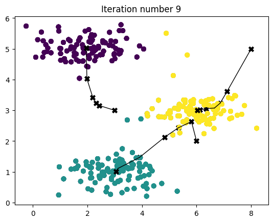
当您运行下面的代码时，它将产生一个可视化图形，展示算法每次迭代的进展情况。

• 最终，您的图形应该看起来像Figure 1中显示的那样。

def run_kMeans(x,initial_centroids,max_iters =10,plot_progress = False):
    #初始化
    m, n = x.shape
    K = initial_centroids.shape[0]
    centroids = initial_centroids
    previous_centroids = centroids
    idx = np.zeros(m)
    # 运行K-means
    for i in range(max_iters):
        #输出过程
        print("K-Means iteration %d/%d" % (i, max_iters-1))
        # 对于 X 中的每个示例，将其分配给最接近的质心
        idx = find_closest_centroids(x, centroids)
        # 绘制过程
        if plot_progress:
            plot_progress_kMeans(x, centroids, previous_centroids, idx, K, i)
            previous_centroids = centroids
        # 计算新的质点
        centroids = compute_centroids(x, idx, K)
    plt.show()
    return centroids, idx

x = load_data()
initial_centroids = np.array([[3,3],[6,2],[8,5]])
K = 3
max_iters = 10

centroids, idx = run_kMeans(x, initial_centroids, max_iters, plot_progress=True)

K-Means iteration 0/9
K-Means iteration 1/9
K-Means iteration 2/9
K-Means iteration 3/9
K-Means iteration 4/9
K-Means iteration 5/9
K-Means iteration 6/9
K-Means iteration 7/9
K-Means iteration 8/9
K-Means iteration 9/9

3 - 随机初始化

为了使您在示例数据集的初始质心分配中看到与“图1”相同的图形，该图形的设计是这样的。在实践中，初始化质心的一个良好策略是从训练集中选择随机样本。

在此练习的这部分中，您应该理解如何实现kMeans_init_centroids函数。

• 代码首先随机洗牌示例的索引（使用np.random.permutation()）。
• 然后，它基于索引的随机排列选择前$K$个示例。
  • 这允许随机选择示例，而不会冒选择相同示例的风险。

def kMeans_init_centroids(x,k):
    # 先将数据随机排列
    randidx = np.random.permutation(x.shape[0])
    # 初始簇取随机排列数组前K个
    centroids = x[randidx[:k]]
    return centroids

np.random.permutation(x.shape[0])

array([ 75,  26, 162, 111, 270,  85,   4, 171, 250, 135,  25, 144, 217,
       130, 136, 104, 143, 126,  50, 196, 148,  45, 272,  10, 175,  49,
       125, 179, 221, 169, 296,   1, 282, 204, 197, 241,  78, 290, 205,
        18,  77, 189, 283,  40, 299, 247,   3,  41, 226,  74,  30,  63,
        22, 249, 281,  16, 102,  20, 147, 245, 214, 211, 201, 122,  53,
       220, 252, 218,  73, 255,  83, 229, 219, 159, 206, 181, 156, 109,
       101, 133, 216,  64, 209, 231, 132,  31,  27,  58,  59, 150,  55,
       225, 110, 149, 103,  91, 273, 105, 295,  33, 277, 224, 268, 182,
       200, 235, 262,  15, 127, 119,  86, 285,  57,  35, 165,  80, 167,
        51, 163, 173, 146,  43,   2, 198, 276,  62, 244, 120, 227, 138,
        96,  48, 236, 258, 203, 240, 199,  82, 195,  68, 246,  92, 188,
       164, 155, 153, 187, 183, 280, 141, 113, 284, 174, 260, 215, 267,
       213,  23, 112, 116, 266,  34,  99, 178, 297, 210, 137,  29,  87,
       117, 230,  21, 288, 145,  44, 191, 192, 168, 121,  60, 271,   0,
       237, 291, 251, 157,  89, 264, 242,  32, 142, 177,  39, 294, 234,
        95, 186,  61,  71,  66,  17, 129,  90, 134, 222,   7,  93,  56,
       265, 298,  52, 176, 128,  70, 152,  98, 139, 261, 208,  11, 124,
       212,  76, 228, 151, 238, 207, 278, 123, 158, 115, 223,  14, 274,
       239, 202,  42,  72,  13, 232, 289, 279, 184, 194,  19, 193,  46,
       114, 108,   9, 286, 180, 248, 154,  37, 166, 257, 292, 293, 269,
       107, 259,  79,  12, 106, 256,  97, 287, 170, 185,   5,   8,  84,
        38,  47,  94,  88,  36, 233,  28, 190, 243, 131,  81,   6, 140,
       160, 253, 172, 118,  69, 161, 254, 263,  65,  67, 275, 100,  54,
        24])

4 - K-means图像压缩

在这个练习中，你将使用K-means算法对图像进行压缩。

• 在直接使用24位颜色表示图像的情况下${}^2$，每个像素都表示为三个8位无符号整数（范围从0到255），指定了红色，绿色和蓝色强度值。这种编码通常称为RGB编码。
• 我们的图片包含成千上万种颜色，在本部分中，您将把颜色数量减少到16种颜色。
• 通过进行此缩减，可以以高效的方式表示（压缩）照片。
• 具体而言，您只需要存储选定16种颜色的RGB值，并且对于图像中的每个像素，您现在只需要存储该位置的颜色索引（仅需要4位即可表示16种可能性）。

在本部分中，您将使用K-means算法来选择用于表示压缩图像的16种颜色。

• 具体而言，您将将原始图像中的每个像素视为数据示例，并使用K-means算法在3维RGB空间中找到最佳聚集（聚类）像素的16种颜色。
• 一旦您已经在图像上计算出聚类中心，您将使用16种颜色来替换原始图像中的像素。

_{本练习中提供的照片归Frank Wouters所有，已获得其许可。}

4.1 数据集

加载图片

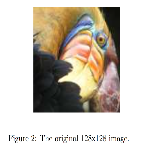
首先，您将使用matplotlib读取原始图像，如下所示。

original_img = plt.imread('bird_small.png')

可视化

plt.imshow(original_img)

<matplotlib.image.AxesImage at 0x25eb49fb640>

​

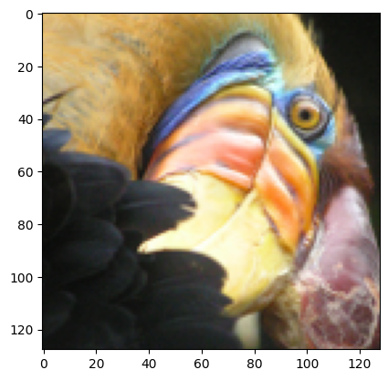
如您所见，这将创建一个三维矩阵original_img，其中

• 前两个索引标识像素位置，
• 第三个索引表示红色、绿色或蓝色。

例如，original_img [50,33,2]给出了行50和列33处像素的蓝色强度。

处理数据

要调用run_kMeans，您需要首先将矩阵original_img转换为二维矩阵。

• 以下代码重新塑造矩阵original_img以创建像素颜色的$m\times 3$矩阵（其中$m=16384=128\times 128$）

# 将所有值除以255，使所有值都在0-1范围内
original_img = original_img / 255

# 重新构造图像成为 m x 3矩阵，其中 m = 128 x 128 = 16384
# 每一行将包含红色、绿色和蓝色像素值
# 这给我们提供了我们将在K-Means上使用的数据集矩阵X_img。

X_img = np.reshape(original_img, (original_img.shape[0] * original_img.shape[1], 3))

4.2图像像素上的 K-mean

现在，运行下面的单元格以在预处理的图像上运行 K-均值。

K = 16
max_iters = 10
initial_centroids = kMeans_init_centroids(X_img,K)

centroids,idx = run_kMeans(X_img,initial_centroids,max_iters)

K-Means iteration 0/9
K-Means iteration 1/9
K-Means iteration 2/9
K-Means iteration 3/9
K-Means iteration 4/9
K-Means iteration 5/9
K-Means iteration 6/9
K-Means iteration 7/9
K-Means iteration 8/9
K-Means iteration 9/9

print("Shape of idx:", idx.shape)
print("Closest centroid for the first five elements:", idx[:5])

Shape of idx: (16384,)
Closest centroid for the first five elements: [7 6 6 7 7]

4.3 压缩图片

找到用于表示图像的前$K=16$种颜色后，现在可以使用find_closest_centroids函数将每个像素位置分配给它最接近的质心。

• 这使您可以使用每个像素的质心赋值来表示原始图像。
• 请注意，您已经大大减少了描述图像所需的位数。
  • 原始图像需要每个$128\times 128$像素位置的24位，因此总大小为$128\times 128\times 24=393,216$位。
  • 新的表示形式需要一些开销的存储，以字典的形式存储16种颜色，每种颜色需要24位，但是图像本身只需要每个像素位置4位。
  • 因此最终使用的位数为$16\times 24+128\times 128\times 4=65,920$位，这相当于将原始图像压缩约6倍。

# 用索引表示图像
X_recovered = centroids[idx, :]
# 将恢复的图像重新调整为正确的维度
X_recovered = np.reshape(X_recovered, original_img.shape)

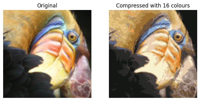
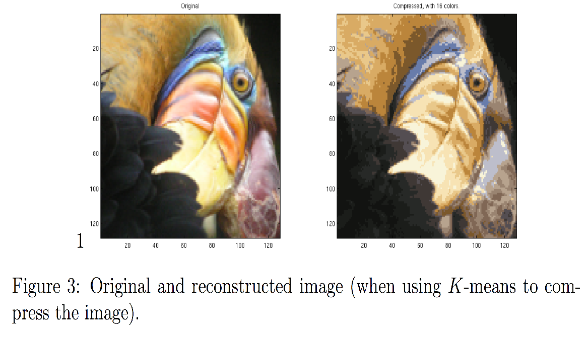
最后，您可以基于仅质心赋值来重新构建图像，以查看压缩的效果。

• 具体而言，您可以将每个像素位置替换为分配给它的质心的均值。
• 图3显示了我们得到的重建图像。即使结果图像保留了大部分原始特征，我们也能看到一些压缩伪影。

fig, ax = plt.subplots(1,2, figsize=(8,8))
plt.axis('off')
# 原始
ax[0].imshow(original_img*255)
ax[0].set_title('Original')
ax[0].set_axis_off()


# 压缩
ax[1].imshow(X_recovered*255)
ax[1].set_title('Compressed with %d colours'%K)
ax[1].set_axis_off()

​