深度学习 -- 张量操作与线性回归 张量的数学运算以及用张量构建线性回归模型

前言

这篇博客继承前篇博客的内容，将对张量的操作进行阐述，同时在理解张量的一些数学的基础上，配合机器学习的理论，在pytorch环境中进行一元线性回归模型的构建。

张量的拼接与切分

torch.cat()
功能：将张量按维度dim进行拼接

torch.stack()
功能：在新创建的维度dim上进行拼接

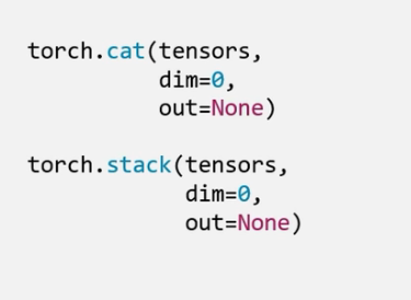
• tensors：张量序列
• dim：要拼接的维度

import torch
a = torch.ones((2,3))
# 张量的拼接
a1 = torch.cat([a,a],dim=0)
print(a)
print(a1)

输出：

tensor([[1., 1., 1.],
        [1., 1., 1.]])
tensor([[1., 1., 1.],
        [1., 1., 1.],
        [1., 1., 1.],
        [1., 1., 1.]])

dim=1

a2 = torch.cat([a,a],dim=1)
print(a2)

tensor([[1., 1., 1., 1., 1., 1.],
        [1., 1., 1., 1., 1., 1.]])

stack：

import torch
a = torch.ones((2,3))

a1 = torch.stack([a,a],dim=2)
print(a1)

输出：

tensor([[[1., 1.],
         [1., 1.],
         [1., 1.]],

        [[1., 1.],
         [1., 1.],
         [1., 1.]]])

torch.chunk()
功能：将张量按维度dim进行平均切分
返回值：张量列表
注意事项：若不能整除，最后一份张量小于其他张量

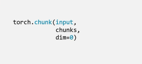
• input：要切分的张量
• chunks：要切分的份数
• dim：要切分的维度

b = torch.ones((2,5))
print(b)
b1 = torch.chunk(b,dim=1,chunks=2)
print(b1)

输出：

tensor([[1., 1., 1., 1., 1.],
        [1., 1., 1., 1., 1.]])
(tensor([[1., 1., 1.],
        [1., 1., 1.]]), tensor([[1., 1.],
        [1., 1.]]))

torch.split()
功能：将张量按维度dim进行切分
返回值：张量列表

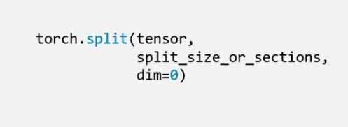
• tensor：要切分的张量
• split_size_or_setions:为int时，表示每一份的长度；为list时，按lisr元素切分
• dim：要切分的维度

c = torch.ones((2,5))
c1 = torch.split(c,2,dim=1)
print(c1)

(tensor([[1., 1.],
        [1., 1.]]), tensor([[1., 1.],
        [1., 1.]]), tensor([[1.],
        [1.]]))

采用list：

c = torch.ones((2,5))
c1 = torch.split(c,[2,1,2],dim=1)
# print(c1)
for i in c1:
    print(i)

tensor([[1., 1.],
        [1., 1.]])
tensor([[1.],
        [1.]])
tensor([[1., 1.],
        [1., 1.]])

注意：
list中所有的元素加起来需要等于指定维度上的张量的长度。

张量的索引

torch.index_select()
功能：在维度dim上，按index索引数据
返回值：依index索引数据拼接的张量

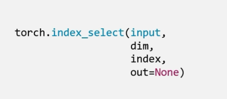
• input:要索引的张量
• dim：要索引的维度
• index：要索引数据的序号

d = torch.randint(0,9,size=(3,3))
idx = torch.tensor([0,2],dtype=torch.long)
d1 = torch.index_select(d,dim=0,index=idx)
print(d)
print(idx)
print(d1)

输出：

tensor([[5, 0, 3],
        [1, 0, 3],
        [0, 8, 2]])
tensor([0, 2])
tensor([[5, 0, 3],
        [0, 8, 2]])

注意：
index的值需要是一个张量 而且dtype也必须是torch.long

torch.masked_select()
功能：按mask中的True进行索引
返回值：一维张量

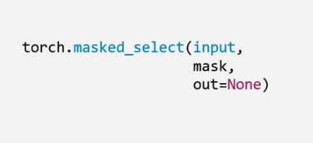
• input:要索引的张量
• mask:与input同形状的布尔类型张量

t = torch.randint(0,9,size=(3,3))
mask = t.ge(5)
print(t)
print(mask)

ge(x)方法的使用：
当张量中的元素>=x的时候就会变True，剩余情况则为False，该例子中x是5.

t和mask的值：（每次都会变）

tensor([[0, 3, 6],
        [7, 5, 8],
        [2, 8, 0]])
tensor([[False, False,  True],
        [ True,  True,  True],
        [False,  True, False]])

使用masked_select(）方法进行布尔值为True的元素索引

t = torch.randint(0,9,size=(3,3))
mask = t.ge(5)
print(t)
print(mask)

t1 = torch.masked_select(t,mask=mask)
print(t1)

输出：

tensor([[8, 8, 4],
        [1, 4, 7],
        [6, 4, 5]])
tensor([[ True,  True, False],
        [False, False,  True],
        [ True, False,  True]])
tensor([8, 8, 7, 6, 5])

张量变换

torch.reshape()
功能：变换张量的形状
注意事项：当张量在内存中是连续时，新张量与input共享数据内存

• input:要变换的张量
• shape:新张量的形状

t = torch.ones(8)
t_reshape = torch.reshape(t,(2,4))
print(t)
print(t_reshape)

输出：

tensor([1., 1., 1., 1., 1., 1., 1., 1.])
tensor([[1., 1., 1., 1.],
        [1., 1., 1., 1.]])

如果把原始张量的第一个元素改为2

t[0] = 2
print(t_reshape)

tensor([[2., 1., 1., 1.],
        [1., 1., 1., 1.]])

会发现改变过形状的张量的第一个元素也会改变，说明新张量与input共享数据内存。

注：共享数据内存不代表，它们在同一个内存地址，而是代表它们所指向的内存空间是一样的。

print(id(t),id(t_reshape)) # 2081724628720 2081889008512
print(id(t.data),id(t_reshape.data)) # 1370880600800 1370880600800

torch.transpose()
功能：交换张量的两个维度

torch.t()
功能：2维张量转置，对矩阵而言，等价于torch.transpose(input,0,1)

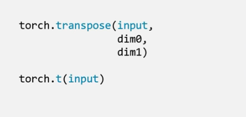
• input:要交换的张量
• dim0：要交换的维度
• dim1：要交换的维度

t = torch.rand(size=(2,3,4))
print(t)
t1 = torch.transpose(t,0,1)
print(t1)

tensor([[[0.6628, 0.1919, 0.1204, 0.3246],
         [0.0973, 0.0540, 0.3222, 0.4540],
         [0.2753, 0.3575, 0.4117, 0.2105]],

        [[0.0800, 0.7416, 0.3095, 0.6480],
         [0.9503, 0.8973, 0.0828, 0.2698],
         [0.6524, 0.1959, 0.3461, 0.8498]]])
tensor([[[0.6628, 0.1919, 0.1204, 0.3246],
         [0.0800, 0.7416, 0.3095, 0.6480]],

        [[0.0973, 0.0540, 0.3222, 0.4540],
         [0.9503, 0.8973, 0.0828, 0.2698]],

        [[0.2753, 0.3575, 0.4117, 0.2105],
         [0.6524, 0.1959, 0.3461, 0.8498]]])

Process finished with exit code 0

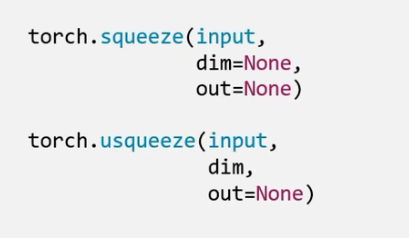
torch.squeeze()
功能：压缩维长度为1的维度（轴）

• dim：若为None，移出所有长度为1 的轴；若指定维度，当且仅当该轴长度为1时，可以被移除；

torch.unsqueeze()
功能：依据dim扩展维度

• dim：扩展的维度

t = torch.rand((1,2,3,1))
print(t.shape)
t1 = torch.squeeze(t)
print(t1.shape)

输出：

torch.Size([1, 2, 3, 1])
torch.Size([2, 3])

如果指定了dim参数：

t = torch.rand((1,2,3,1))
print(t.shape)
t1 = torch.squeeze(t,dim=0)
print(t1.shape)

输出：

torch.Size([1, 2, 3, 1])
torch.Size([2, 3, 1])

就只会压缩第四维度的轴。

张量的数学运算

pytorch中提供了丰富的张量数学运算

1、加减乘除

• torch.add()
• torch.addcdiv()
• torch.addcmul()
• torch.sub()
• torch.div()
• torch.mul()

2、对数，指数，幂函数

• torch.log(input,out=None)
• torch.log10(input,out=None)
• torch.log2(input,out=None)
• torch.exp(input,out=None)
• torch.pow()

3、三角函数

• torch.abs(input,out=None)
• torch.acos(input,out=None)
• torch.cosh(input,out=None)
• torch.cos(input,out=None)
• torch.asin(input,out=None)
• torch.atan(input,out=None)
• torch.atan2(input,out=None)

torch.add()
功能：逐元素计算 input + alpha x other

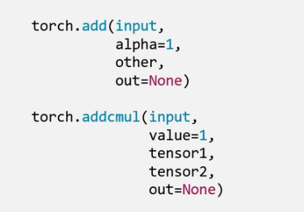
• input:第一个张量
• alpha:乘项因子
• other:第二个张量

add()方法不仅仅可以做加法运算，还可以做线性运算

• 机器学习中的公式：
  y = wx + b

import torch
# torch.add()

t = torch.rand((3,3))
t1 = torch.rand((3,3))
print("t",t)
print("t1",t1)
t2 = torch.add(t,t1)
t3 = torch.add(t,t1,alpha=2)
print("t2",t2)
print("t3",t3)

输出：

t tensor([[0.8218, 0.8576, 0.4829],
        [0.6046, 0.1290, 0.4835],
        [0.5752, 0.2386, 0.1260]])
t1 tensor([[0.5306, 0.7424, 0.4328],
        [0.3278, 0.1980, 0.4354],
        [0.4742, 0.4319, 0.8922]])
t2 tensor([[1.3524, 1.6000, 0.9157],
        [0.9324, 0.3270, 0.9189],
        [1.0494, 0.6705, 1.0182]])
t3 tensor([[1.8830, 2.3423, 1.3484],
        [1.2602, 0.5249, 1.3544],
        [1.5236, 1.1024, 1.9104]])

线性回归

线性回归时分析一个变量与另外一（多）个变量之间关系的 方法

因变量：y
自变量：x
关系：线性

y = wx + b

分析：求解w，b

求解步骤：
1、确定模型
Model: y = wx + b

2、选择损失函数
MSE: 均方差

3、求解梯度并更新w，b
w = w - LRw.grad
b = b - LRw.grad

pytorch中实现一元线性回归模型

# 一元线性回归
import torch
import matplotlib.pyplot as plt

torch.manual_seed(10)

lr = 0.1 #学习率/步长

# 创建训练数据
x = torch.rand(20,1) * 10
y = 2*x + (5 + torch.randn(20,1))

# 构建线性回归参数
w = torch.randn((1),requires_grad=True) # 允许更新梯度
b = torch.zeros((1),requires_grad=True)

for iteration in range(1000):
    # 前向传播
    wx = torch.mul(w,x)
    y_pred = torch.add(wx,b)

    # 计算MSE loss
    loss = (0.5*(y-y_pred)**2).mean()

    # 反向传播
    loss.backward()

    # 更新参数
    w.data.sub_(lr * w.grad)
    b.data.sub_(lr * b.grad)

    if iteration % 20 == 0:
        plt.scatter(x.data.numpy(),y.data.numpy())
        plt.plot(x.data.numpy(),y_pred.data.numpy(),'r-',lw=5)
        plt.text(2,20,'Loss=%.4f' % loss.data.numpy())
        plt.xlim(1.5,10)
        plt.ylim(8,28)
        plt.title("huiguimoxing interation={}".format(iteration))
        plt.pause(0.5)
        plt.show()

        if loss.data.numpy() < 1:
            break

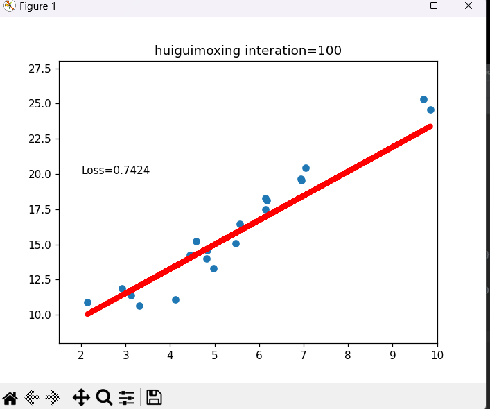
当迭代到100次时loss已经接近0了 此时该线性的图也接近这些这些数据。