一、GoogLeNet网络模型架构
论文出处:Going deeper with convolutions
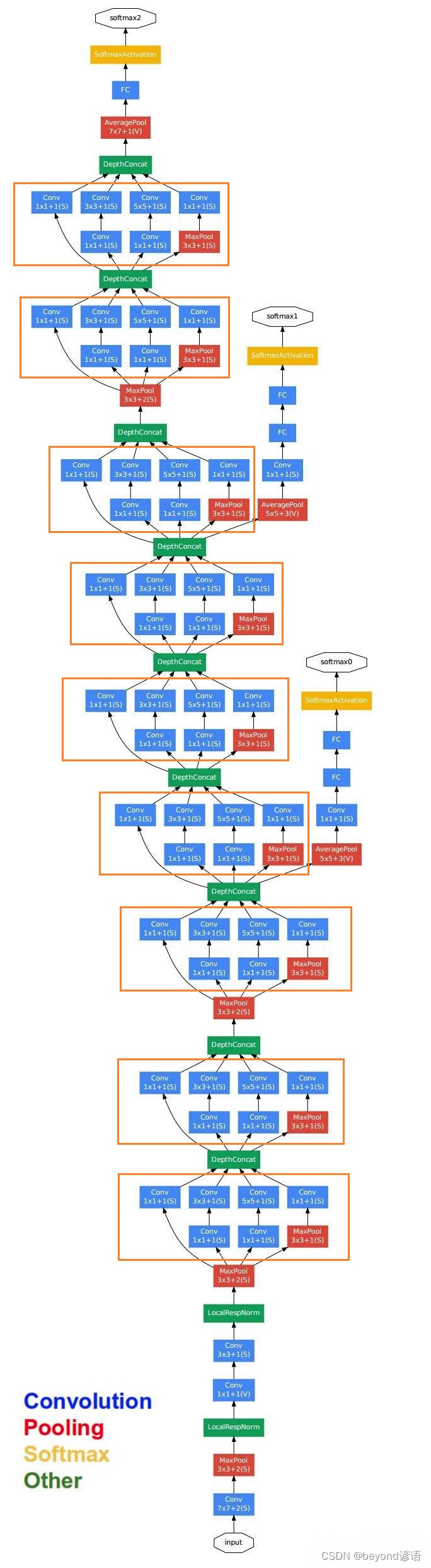
很容易发现里面有很多复用单元,把这些重复的单元封装成一个类,到时候调用即可,这样的复用单元在论文中被称为Inception module
二、复合模块实现
这里以论文中的(b) Inception module with dimension reductions为例进行简单复现
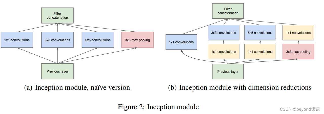
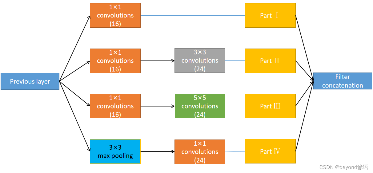
为了方便观察结构,将模块进行适当的转换
之所以这样做,其目的初衷在于通过各种方法都进行尝试,最终确定出最优的解
四个路径算出来了,之后按通道方向进行拼接,因为大小都一致,除了通道不一样而已
1×1的卷积作用
卷积核大小为1×1,卷积核的通道数取决于输入张量的通道数,卷积核的个数取决于输出张量的通道数
不管输入特征的通道数是多少,做完卷积最后都会变成通道数为1
1×1的卷积最主要的作用是:改变通道数的数量、降低运算量
举例:

使用5×5的卷积的话,所需参数为:
卷积核表面5×5的卷积,每个元素都得进行对应相乘28×28,深度为192,最终输出的深度为32
最终5*5*28*28*192*32 = 120422400
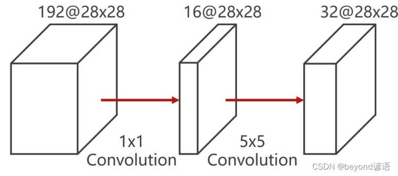
首先使用1×1的卷积,改变通道数,然后再使用5×5的卷积
第一个卷积核表面1×1的卷积,每个元素都得进行对应相乘再相加操作28×28,深度为192
第二个卷积核表面5×5的卷积,每个元素都得进行对应相乘再相加操作28×28,深度为16
最终1*1*18*18*192*16 + 5*5*28*28*16*32 = 12433648
差不只有原来的十分之一参数量
数据集还是选用MNIST手写数字数据集,详细的使用可参考博文:九、多分类问题
import torch
from torchvision import transforms
from torchvision import datasets
from torch.utils.data import DataLoader
import torch.nn.functional as F #为了使用relu激活函数
import torch.optim as optim

batch_size = 64
transform = transforms.Compose([
    transforms.ToTensor(),#把图片变成张量形式
    transforms.Normalize((0.1307,),(0.3081,)) #均值和标准差进行数据标准化,这俩值都是经过整个样本集计算过的
])

train_dataset = datasets.MNIST(root='./',train=True,download=True,transform = transform)
train_loader = DataLoader(train_dataset,shuffle=True,batch_size=batch_size)

test_dataset = datasets.MNIST(root="./",train=False,download=True,transform=transform)
test_loader = DataLoader(test_dataset,shuffle=False,batch_size=batch_size)
为了测试模型,使用测试集中的第1张作为测试样本进行调试
由x.shape得到样本的形状为[1, 28, 28],但pytorch中的卷积层函数调用需要传入的样本格式为[B,C,W,H],故通过x.view(-1,1,28,28)转换格式,得到最终的测试样本x,其形状为[1, 1, 28, 28]
x,y = test_dataset[0]
x.shape
"""
torch.Size([1, 28, 28])
"""
y
"""
7
"""

x = x.view(-1,1,28,28)
x.shape
"""
torch.Size([1, 1, 28, 28])
"""
由上图的复用模块可知,其由四部分组成,接下来开始对这四个部分一一进行实现
1、调试
①Part Ⅰ
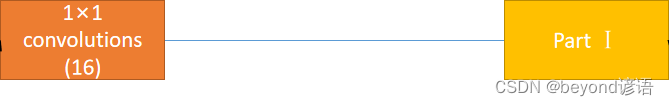
第一部分是卷积层,输出通道数为16,卷积核的大小为1×1
因为样本形状为torch.Size([1, 1, 28, 28]),[B,C,W,H],故通过in_channel = x.shape[1]获取输入通道数
根据需要构建卷积层part_1_conv = torch.nn.Conv2d(in_channels=in_channel,out_channels=16,kernel_size=1)
in_channel = x.shape[1]
part_1_conv = torch.nn.Conv2d(in_channels=in_channel,out_channels=16,kernel_size=1)
part_1 = part_1_conv(x)
part_1.shape
"""
torch.Size([1, 16, 28, 28])
"""
②Part Ⅱ
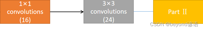
第二部分是先进行卷积核大小为1×1的卷积层,输出通道数为16;然后再来个卷积核为3×3的卷积层,输出通道数为24
因为样本形状为torch.Size([1, 1, 28, 28]),[B,C,W,H],故通过in_channel = x.shape[1]获取输入通道数
根据需要构建第一个卷积层
part_2_conv1 = torch.nn.Conv2d(in_channels=in_channel,out_channels=16,kernel_size=1)
在构建第二个卷积层的时候,为了保证特征图大小不变,进行了加边
part_2_conv2 = torch.nn.Conv2d(in_channels=16,out_channels=24,kernel_size=3,padding=1)
in_channel = x.shape[1]
part_2_conv1 = torch.nn.Conv2d(in_channels=in_channel,out_channels=16,kernel_size=1)
part_2_conv2 = torch.nn.Conv2d(in_channels=16,out_channels=24,kernel_size=3,padding=1)
part_2 = part_2_conv1(x)
part_2 = part_2_conv2(part_2)
part_2.shape
"""
torch.Size([1, 24, 28, 28])
"""
③Part Ⅲ
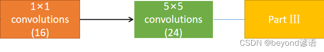
第三部分是先进行卷积核大小为1×1的卷积层,输出通道数为16;然后再来个卷积核为5×5的卷积层,输出通道数为24
因为样本形状为torch.Size([1, 1, 28, 28]),[B,C,W,H],故通过in_channel = x.shape[1]获取输入通道数
根据需要构建第一个卷积层
part_3_conv1 = torch.nn.Conv2d(in_channels=in_channel,out_channels=16,kernel_size=1)
在构建第二个卷积层的时候,为了保证特征图大小不变,进行了加边
part_3_conv2 = torch.nn.Conv2d(in_channels=16,out_channels=24,kernel_size=5,padding=2)
in_channel = x.shape[1]
part_3_conv1 = torch.nn.Conv2d(in_channels=in_channel,out_channels=16,kernel_size=1)
part_3_conv2 = torch.nn.Conv2d(in_channels=16,out_channels=24,kernel_size=5,padding=2)
part_3 = part_3_conv1(x)
part_3 = part_3_conv2(part_3)
part_3.shape
"""
torch.Size([1, 24, 28, 28])
"""
④Part Ⅳ
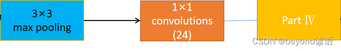
第四部分是先进行卷积核大小为3×3的最大池化层;然后再来个卷积核为1×1的卷积层,输出通道数为24
因为样本形状为torch.Size([1, 1, 28, 28]),[B,C,W,H],故通过in_channel = x.shape[1]获取输入通道数
根据需要构建最大池化层,为了保证输出特征大小一致,stride设置为1(默认情况下与kernel一致),padding设置为1
part_4_maxpool = torch.nn.MaxPool2d(kernel_size=3,stride=1,padding=1)
根据需要构建卷积层
part_4_conv = torch.nn.Conv2d(in_channels=in_channel,out_channels=24,kernel_size=1)
in_channel = x.shape[1]
part_4_maxpool = torch.nn.MaxPool2d(kernel_size=3,stride=1,padding=1)
part_4_conv = torch.nn.Conv2d(in_channels=in_channel,out_channels=24,kernel_size=1)
part_4 = part_4_maxpool(x)
part_4 = part_4_conv(part_4)
part_4.shape
"""
torch.Size([1, 24, 28, 28])
"""
⑤合并
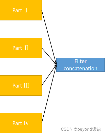
每层的结果都拿到之后,进行troch.cat()根据通道进行合并,因为只有通道数不相同,其他的都完全一致
[B,C,W,H]通道数在第二个,故dim=1
print(part_1.shape)
print(part_2.shape)
print(part_3.shape)
print(part_4.shape)
"""
torch.Size([1, 16, 28, 28])
torch.Size([1, 24, 28, 28])
torch.Size([1, 24, 28, 28])
torch.Size([1, 24, 28, 28])
"""

outputs = [part_1,part_2,part_3,part_4]
final = torch.cat(outputs,dim=1)#因为是[B,C,W,H],通道数是1,故dim=1
final.shape# 16+24+24+24=88
"""
torch.Size([1, 88, 28, 28])
"""
2、封装
根据上述的调试,将各层进行封装
class Google_Net (torch.nn.Module):
    def __init__(self,in_channel):
        super(Google_Net ,self).__init__()

        self.part_1_conv = torch.nn.Conv2d(in_channels=in_channel,out_channels=16,kernel_size=1)

        self.part_2_conv1 = torch.nn.Conv2d(in_channels=in_channel,out_channels=16,kernel_size=1)
        self.part_2_conv2 = torch.nn.Conv2d(in_channels=16,out_channels=24,kernel_size=3,padding=1)

        self.part_3_conv1 = torch.nn.Conv2d(in_channels=in_channel,out_channels=16,kernel_size=1)
        self.part_3_conv2 = torch.nn.Conv2d(in_channels=16,out_channels=24,kernel_size=5,padding=2)

        self.part_4_maxpool = torch.nn.MaxPool2d(kernel_size=3,stride=1,padding=1)
        self.part_4_conv = torch.nn.Conv2d(in_channels=in_channel,out_channels=24,kernel_size=1)

    def forward(self,x):
        part_1 = self.part_1_conv(x)

        part_2 = self.part_2_conv1(x)
        part_2 = self.part_2_conv2(part_2)

        part_3 = self.part_3_conv1(x)
        part_3 = self.part_3_conv2(part_3)

        part_4 = self.part_4_maxpool(x)
        part_4 = self.part_4_conv(part_4)

        outputs = [part_1,part_2,part_3,part_4]
        final = torch.cat(outputs,dim=1)

        return final
还是使用上述的x进行测试一下
in_channel = x.shape[1]
model = Google_Net (in_channel)
model(x).shape
"""
torch.Size([1, 88, 28, 28])
"""
对着了,跟上述的调试结果一样,嘿嘿
3、模型整体架构
按下列需求对模型架构进行复现
①准备数据集
老规矩:MNIST手写数字数据集
上述都有简单介绍,这里就不再赘述
②加载数据集
import torch
from torchvision import transforms
from torchvision import datasets
from torch.utils.data import DataLoader
import torch.nn.functional as F #为了使用relu激活函数
import torch.optim as optim

batch_size = 64
transform = transforms.Compose([
    transforms.ToTensor(),#把图片变成张量形式
    transforms.Normalize((0.1307,),(0.3081,)) #均值和标准差进行数据标准化,这俩值都是经过整个样本集计算过的
])

train_dataset = datasets.MNIST(root='./',train=True,download=True,transform = transform)
train_loader = DataLoader(train_dataset,shuffle=True,batch_size=batch_size)

test_dataset = datasets.MNIST(root="./",train=False,download=True,transform=transform)
test_loader = DataLoader(test_dataset,shuffle=False,batch_size=batch_size)
测试一下
x,y = test_dataset[1]
x.shape
"""
torch.Size([1, 28, 28])
"""
y
"""
2
"""
x = x.view(-1,1,28,28)
x.shape#[B,C,W,H]
"""
torch.Size([1, 1, 28, 28])
"""
in_channel = x.shape[1]
in_channel
"""
1
"""
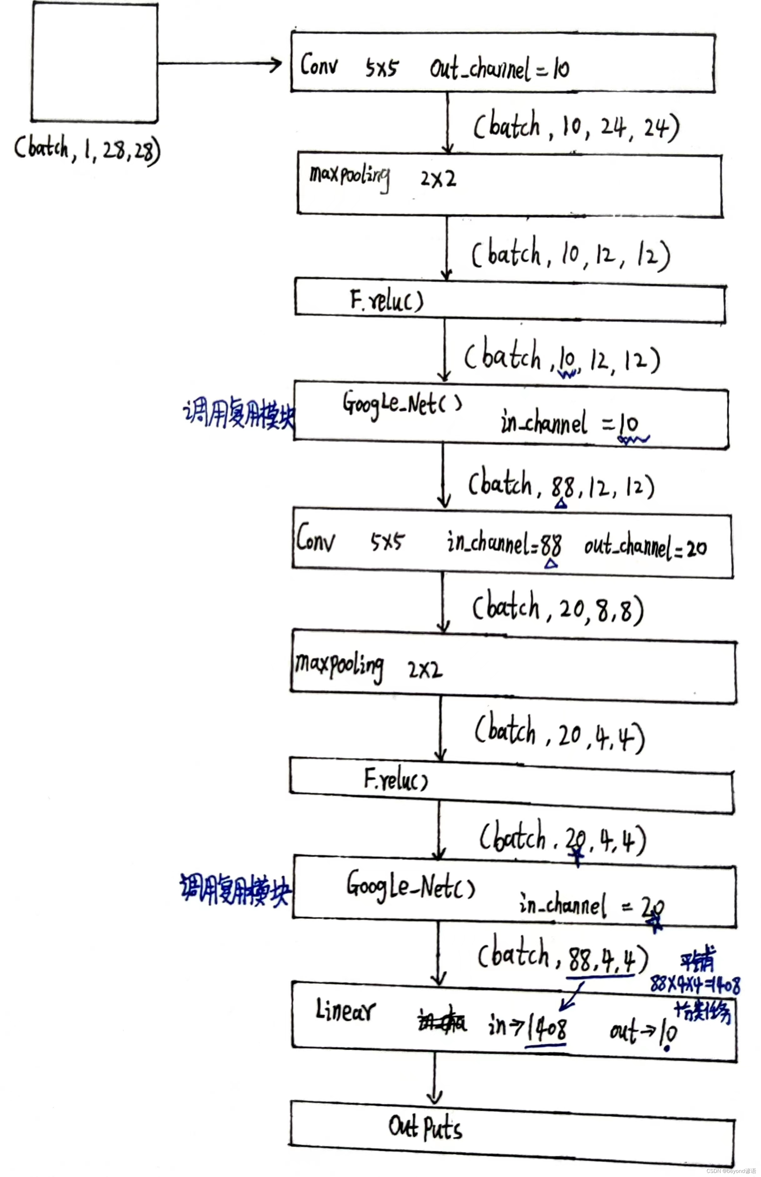
③模型构建
根据上述需求,进行调试搭建
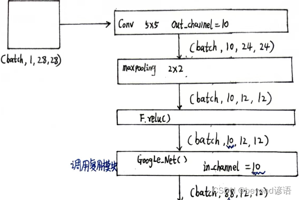
这里的Google_Net部分结构使用上面所构建的模型架构
conv1 = torch.nn.Conv2d(in_channels=in_channel,out_channels=10,kernel_size=5)
maxpooling = torch.nn.MaxPool2d(2)

conv_1 = conv1(x)
conv_1.shape
"""
torch.Size([1, 10, 24, 24])
"""

maxpool = maxpooling(conv_1)
maxpool.shape
"""
torch.Size([1, 10, 12, 12])
"""

relu = F.relu(maxpool)
relu.shape
"""
torch.Size([1, 10, 12, 12])
"""

google = Google_Net(in_channel=10)
next1 = google(relu)
next1.shape
"""
torch.Size([1, 88, 12, 12])
"""
根据输出结果可知,结果一致,next
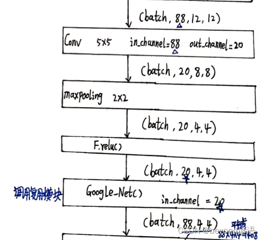
in_channel = next1.shape[1]#得到出入特征的通道
conv2 = torch.nn.Conv2d(in_channels=in_channel,out_channels=20,kernel_size=5)
maxpooling = torch.nn.MaxPool2d(2)


conv_2 = conv2(next1)
conv_2.shape
"""
torch.Size([1, 20, 8, 8])
"""

maxpool2 = maxpooling(conv_2)
maxpool2.shape
"""
torch.Size([1, 20, 4, 4])
"""

relu2 = F.relu(maxpool2)
relu2.shape
"""
torch.Size([1, 20, 4, 4])
"""

google2 = Google_Net(in_channel=20)
next2 = google2(relu2)
next2.shape
"""
torch.Size([1, 88, 4, 4])
"""
根据输出结果可知,结果一致,next
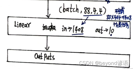
最后是全连接层,得先获取到next2全部参数个数,然后view一下,最后输出10分类即可
all_para = next2.shape[0] * next2.shape[1] * next2.shape[2] * next2.shape[3]
all_para
"""
1408
"""
batch_size = x.shape[0]
final = next2.view(batch_size,-1)
linear = torch.nn.Linear(all_para,10)
final = linear(final)
final.shape
"""
torch.Size([1, 10])
"""
完整模型实现
class y_net(torch.nn.Module):
    def __init__(self):
        super(y_net,self).__init__()

        self.conv1 = torch.nn.Conv2d(in_channels=1,out_channels=10,kernel_size=5)
        self.maxpooling = torch.nn.MaxPool2d(2)
        self.google = Google_Net(in_channel=10)
        self.conv2 = torch.nn.Conv2d(in_channels=88,out_channels=20,kernel_size=5)
        self.google2 = Google_Net(in_channel=20)
        self.linear = torch.nn.Linear(1408,10)

    def forward(self,x):
        batch_size = x.shape[0]

        conv_1 = self.conv1(x)
        maxpool = self.maxpooling(conv_1)
        relu = F.relu(maxpool)
        next1 = self.google(relu)

        conv_2 = self.conv2(next1)
        maxpool2 = self.maxpooling(conv_2)
        relu2 = F.relu(maxpool2)
        next2 = self.google2(relu2)

        final = next2.view(batch_size,-1)
        final = linear(final)

        return final


class Google_Net(torch.nn.Module):
    def __init__(self,in_channel):
        super(Google_Net ,self).__init__()

        self.part_1_conv = torch.nn.Conv2d(in_channels=in_channel,out_channels=16,kernel_size=1)

        self.part_2_conv1 = torch.nn.Conv2d(in_channels=in_channel,out_channels=16,kernel_size=1)
        self.part_2_conv2 = torch.nn.Conv2d(in_channels=16,out_channels=24,kernel_size=3,padding=1)

        self.part_3_conv1 = torch.nn.Conv2d(in_channels=in_channel,out_channels=16,kernel_size=1)
        self.part_3_conv2 = torch.nn.Conv2d(in_channels=16,out_channels=24,kernel_size=5,padding=2)

        self.part_4_maxpool = torch.nn.MaxPool2d(kernel_size=3,stride=1,padding=1)
        self.part_4_conv = torch.nn.Conv2d(in_channels=in_channel,out_channels=24,kernel_size=1)

    def forward(self,x):
        part_1 = self.part_1_conv(x)

        part_2 = self.part_2_conv1(x)
        part_2 = self.part_2_conv2(part_2)

        part_3 = self.part_3_conv1(x)
        part_3 = self.part_3_conv2(part_3)

        part_4 = self.part_4_maxpool(x)
        part_4 = self.part_4_conv(part_4)

        outputs = [part_1,part_2,part_3,part_4]
        final = torch.cat(outputs,dim=1)

        return final
测试一下
x,y = test_dataset[5]
x = x.view(-1,1,28,28)
model = y_net()
yy = model(x)
yy.shape
"""
torch.Size([1, 10])
"""
其他的部分详细可参考博文:十、CNN卷积神经网络实战
④损失函数和优化器
lossf = torch.nn.CrossEntropyLoss()
optimizer = optim.SGD(model.parameters(),lr=0.0001,momentum=0.5)
⑤训练函数构建
def ytrain(epoch):
    loss_total = 0.0
    for batch_index ,data in enumerate(train_loader,0):
        x,y = data
        #x,y = x.to(device), y.to(device)#GPU加速
        optimizer.zero_grad()

        y_hat = model(x)
        loss = lossf(y_hat,y)
        loss.backward()
        optimizer.step()

        loss_total += loss.item()
        if batch_index % 300 == 299:# 每300epoch输出一次
            print("epoch:%d, batch_index:%5d \t loss:%.3f"%(epoch+1, batch_index+1, loss_total/300))
            loss_total = 0.0 #每次epoch都将损失清除
⑥测试函数构建
def ytest():
    correct = 0#模型预测正确的数量
    total = 0#样本总数
    with torch.no_grad():#测试不需要梯度,减小计算量
        for data in test_loader:#读取测试样本数据
            images, labels = data
            #images, labels = images.to(device), labels.to(device) #GPU加速
            pred = model(images)#预测,每一个样本占一行,每行有十个值,后续需要求每一行中最大值所对应的下标
            pred_maxvalue, pred_maxindex = torch.max(pred.data,dim=1)#沿着第一个维度,一行一行来,去找每行中的最大值,返回每行的最大值和所对应下标
            total += labels.size(0)#labels是一个(N,1)的向量,对应每个样本的正确答案
            correct += (pred_maxindex == labels).sum().item()#使用预测得到的最大值的索引和正确答案labels进行比较,一致就是1,不一致就是0
        print("Accuracy on testset :%d %%"%(100*correct / total))#correct预测正确的样本个数 / 样本总数 * 100 = 模型预测正确率
⑦主函数调用
if __name__ == '__main__':
    for epoch in range(10):#训练10次
        ytrain(epoch)#训练一次
        if epoch%10 == 9:
            ytest()#训练10次,测试1次
⑧完整代码
import torch
from torchvision import transforms
from torchvision import datasets
from torch.utils.data import DataLoader
import torch.nn.functional as F #为了使用relu激活函数
import torch.optim as optim

batch_size = 64
transform = transforms.Compose([
    transforms.ToTensor(),#把图片变成张量形式
    transforms.Normalize((0.1307,),(0.3081,)) #均值和标准差进行数据标准化,这俩值都是经过整个样本集计算过的
])

train_dataset = datasets.MNIST(root='./',train=True,download=True,transform = transform)
train_loader = DataLoader(train_dataset,shuffle=True,batch_size=batch_size)

test_dataset = datasets.MNIST(root="./",train=False,download=True,transform=transform)
test_loader = DataLoader(test_dataset,shuffle=False,batch_size=batch_size)

class y_net(torch.nn.Module):
    def __init__(self):
        super(y_net,self).__init__()

        self.conv1 = torch.nn.Conv2d(in_channels=1,out_channels=10,kernel_size=5)
        self.maxpooling = torch.nn.MaxPool2d(2)
        self.google = Google_Net(in_channel=10)
        self.conv2 = torch.nn.Conv2d(in_channels=88,out_channels=20,kernel_size=5)
        self.google2 = Google_Net(in_channel=20)
        self.linear = torch.nn.Linear(1408,10)

    def forward(self,x):
        batch_size = x.shape[0]

        conv_1 = self.conv1(x)
        maxpool = self.maxpooling(conv_1)
        relu = F.relu(maxpool)
        next1 = self.google(relu)

        conv_2 = self.conv2(next1)
        maxpool2 = self.maxpooling(conv_2)
        relu2 = F.relu(maxpool2)
        next2 = self.google2(relu2)

        final = next2.view(batch_size,-1)
        final = self.linear(final)

        return final


class Google_Net(torch.nn.Module):
    def __init__(self,in_channel):
        super(Google_Net ,self).__init__()

        self.part_1_conv = torch.nn.Conv2d(in_channels=in_channel,out_channels=16,kernel_size=1)

        self.part_2_conv1 = torch.nn.Conv2d(in_channels=in_channel,out_channels=16,kernel_size=1)
        self.part_2_conv2 = torch.nn.Conv2d(in_channels=16,out_channels=24,kernel_size=3,padding=1)

        self.part_3_conv1 = torch.nn.Conv2d(in_channels=in_channel,out_channels=16,kernel_size=1)
        self.part_3_conv2 = torch.nn.Conv2d(in_channels=16,out_channels=24,kernel_size=5,padding=2)

        self.part_4_maxpool = torch.nn.MaxPool2d(kernel_size=3,stride=1,padding=1)
        self.part_4_conv = torch.nn.Conv2d(in_channels=in_channel,out_channels=24,kernel_size=1)

    def forward(self,x):
        part_1 = self.part_1_conv(x)

        part_2 = self.part_2_conv1(x)
        part_2 = self.part_2_conv2(part_2)

        part_3 = self.part_3_conv1(x)
        part_3 = self.part_3_conv2(part_3)

        part_4 = self.part_4_maxpool(x)
        part_4 = self.part_4_conv(part_4)

        outputs = [part_1,part_2,part_3,part_4]
        final = torch.cat(outputs,dim=1)

        return final

model = y_net()
lossf = torch.nn.CrossEntropyLoss()
optimizer = optim.SGD(model.parameters(),lr=0.0001,momentum=0.5)


def ytrain(epoch):
    loss_total = 0.0
    for batch_index ,data in enumerate(train_loader,0):
        x,y = data
        #x,y = x.to(device), y.to(device)#GPU加速
        optimizer.zero_grad()

        y_hat = model(x)
        loss = lossf(y_hat,y)
        loss.backward()
        optimizer.step()

        loss_total += loss.item()
        if batch_index % 300 == 299:# 每300epoch输出一次
            print("epoch:%d, batch_index:%5d \t loss:%.3f"%(epoch+1, batch_index+1, loss_total/300))
            loss_total = 0.0 #每次epoch都将损失清除


def ytest():
    correct = 0#模型预测正确的数量
    total = 0#样本总数
    with torch.no_grad():#测试不需要梯度,减小计算量
        for data in test_loader:#读取测试样本数据
            images, labels = data
            #images, labels = images.to(device), labels.to(device) #GPU加速
            pred = model(images)#预测,每一个样本占一行,每行有十个值,后续需要求每一行中最大值所对应的下标
            pred_maxvalue, pred_maxindex = torch.max(pred.data,dim=1)#沿着第一个维度,一行一行来,去找每行中的最大值,返回每行的最大值和所对应下标
            total += labels.size(0)#labels是一个(N,1)的向量,对应每个样本的正确答案
            correct += (pred_maxindex == labels).sum().item()#使用预测得到的最大值的索引和正确答案labels进行比较,一致就是1,不一致就是0
        print("Accuracy on testset :%d %%"%(100*correct / total))#correct预测正确的样本个数 / 样本总数 * 100 = 模型预测正确率


if __name__ == '__main__':
    for epoch in range(10):#训练10次
        ytrain(epoch)#训练一次
        if epoch%10 == 9:
            ytest()#训练10次,测试1次