【文献阅读】Cascaded Partial Decoder for Fast and Accurate Salient Object Detection

写在前面

这是2019CVPR的一篇文章，关于显著目标检测的。提出了一种CPD框架
大概记录一下对这个文章的理解，做了一些图，如有不对，欢迎指正
文章链接：论文下载
代码地址：CPD代码

整体框架

这篇文章的模型是基于VGG16设计的

VGG16分为五个阶段

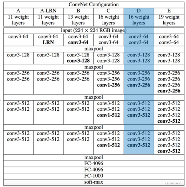
我们先说一下本文的网络模型的整体结构：

将VGG16这五个阶段得到的特征图，分别表示为$f_i=f_1,f_2,f_3,f_4,f_5$，大小为$H/2^{(i-1)},W/2^{(i-1)}$

作者设计了一种分支网络，利用最后两个卷积块构造了两个分支（注意力分支和检测分支）

这是作者给出的网络结构

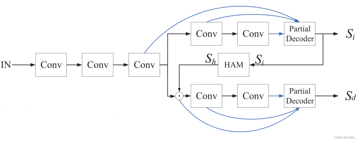
上面是注意力分支，下面是检测分支。

在注意力分支作者设计了一个部分解码器partial decoder 来集成后三层卷积块$f_3,f_4,f_5$提取的特征

经过这个部分解码器，生成了初始的显著图像$S_i$。

我们把这个部分解码器叫做$D_a=g_a(f_3^a,f_4^a,f_5^a)$，解码器输出$S_i$

$S_i$再经过一个整体注意力模块（holistic attention module,HAM）后，得到一个增强的特征$S_h$

作者说，“我们可以通过整合三层特征来获得相对精确的显著图，因此Sh有效地消除了特征f3中的干扰”

$S_h$将用来在下面的检测分支细化特征$f_3$

然后我们将特征图$f_3$与$S_h$按元素相乘，得到检测分支的细化特征$f_3^d=f_3\odot S_h$

同理，将$f_4$与$S_h$按元素相乘，得到$f_4^d=f_4\odot S_h$

将$f_5$与$S_h$按元素相乘，得到$f_5^d=f_5\odot S_h$

我们为检测分支构造另一个部分解码器$D_d=g_d(f_3^d,f_4^d,f_5^d)$，这个解码器输出最终的显著图像$S_d$

使用ground truth联合训练两个分支，两个分支参数不共享。

这就是网络的整体结构和处理流程

下面我们主要详细说下两个部分解码器（partial decoder）和整体注意力模块（holistic attention module,HAM）

部分解码器

这个部分解码器，主要目的就是快速的集成三个块得到的特征图，这里作者设计了一个上下文模块conext module

主要借鉴于这篇论文

• Receptive Field Block Net for Accurate and Fast Object Detection

这篇文章是ECCV2018年，主要贡献就是提出了RFB（Receptive Field Block）

出发点是模拟人类视觉的感受野从而加强网络的特征提取能力

做法就是将特征图通过不同卷积分支，最后再合并不同分支的结果，然后再与特征图合并。

网络结构如下图所示：

就是在ReLU之前，通过这个模块，增加感受野

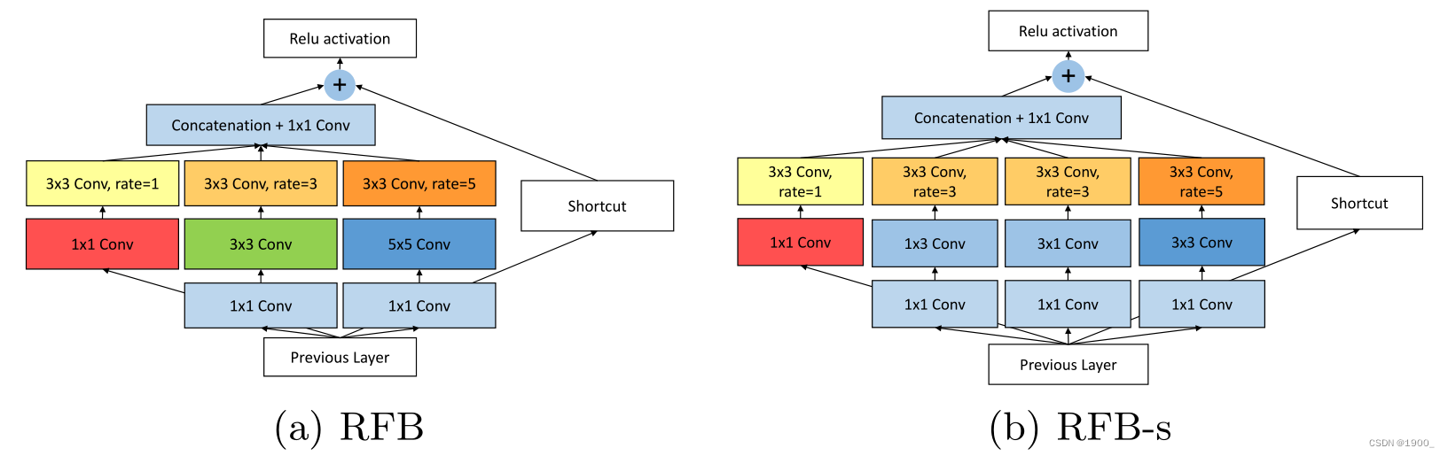
左边的结构是原始的RFB，右边的结构相比RFB把3×3的conv变成了两个1×3和3×1的分支，一是减少了参数量，二是增加了更小的感受野，这样也是在模拟人类视觉系统，捕捉更小的感受野。

而本文作者在原有的RFB基础上增加了一个分支。

我画了个图

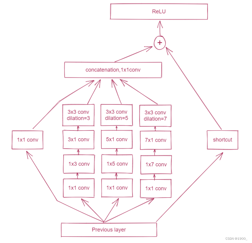
代码如下：

class RFB(nn.Module):
    def __init__(self, in_channel, out_channel):
        super(RFB, self).__init__()
        self.relu = nn.ReLU(True)
        self.branch0 = nn.Sequential(
            nn.Conv2d(in_channel, out_channel, 1),
        )
        self.branch1 = nn.Sequential(
            nn.Conv2d(in_channel, out_channel, 1),
            nn.Conv2d(out_channel, out_channel, kernel_size=(1, 3), padding=(0, 1)),
            nn.Conv2d(out_channel, out_channel, kernel_size=(3, 1), padding=(1, 0)),
            nn.Conv2d(out_channel, out_channel, 3, padding=3, dilation=3)
        )
        self.branch2 = nn.Sequential(
            nn.Conv2d(in_channel, out_channel, 1),
            nn.Conv2d(out_channel, out_channel, kernel_size=(1, 5), padding=(0, 2)),
            nn.Conv2d(out_channel, out_channel, kernel_size=(5, 1), padding=(2, 0)),
            nn.Conv2d(out_channel, out_channel, 3, padding=5, dilation=5)
        )
        self.branch3 = nn.Sequential(
            nn.Conv2d(in_channel, out_channel, 1),
            nn.Conv2d(out_channel, out_channel, kernel_size=(1, 7), padding=(0, 3)),
            nn.Conv2d(out_channel, out_channel, kernel_size=(7, 1), padding=(3, 0)),
            nn.Conv2d(out_channel, out_channel, 3, padding=7, dilation=7)
        )
        self.conv_cat = nn.Conv2d(4*out_channel, out_channel, 3, padding=1)
        self.conv_res = nn.Conv2d(in_channel, out_channel, 1)

        for m in self.modules():
            if isinstance(m, nn.Conv2d):
                m.weight.data.normal_(std=0.01)
                m.bias.data.fill_(0)

    def forward(self, x):
        x0 = self.branch0(x)
        x1 = self.branch1(x)
        x2 = self.branch2(x)
        x3 = self.branch3(x)

        x_cat = torch.cat((x0, x1, x2, x3), 1)
        x_cat = self.conv_cat(x_cat)

        x = self.relu(x_cat + self.conv_res(x))
        return x

回到我们的论文中，VGG16后三个卷积块提取的特征，首先全部经过一个RFB，然后再送入我们的部分解码器

这个部分解码器具体做了些什么呢？

首先，VGG16的五个块每次通过池化都会让图像的尺寸减半。

参考文章：https://blog.csdn.net/qq_42012782/article/details/123222042

但是本论文中使用的VGG是修改过的

池化层放在卷积块的前面，并且第一个卷积块不池化。

具体的可以去看代码，此处只要知道

假设输入图片是WxW，第一个块输出尺寸等于原尺寸，第二个块原尺寸的1/2，第三个块是1/4，第四个块是1/8，第五个块是1/16

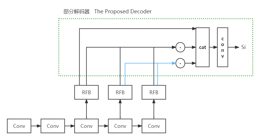
这个部分解码器，就是将x5,x4,x3拿出来。

• 将x5记作x_1

• 将x5与x4相乘，记作x_2。

• 再将x5，x4，x3三个相乘，记作x_3。

• 最后将三个特征cat起来

• 然后经过两个卷积输出一张显著图像。

如果大小不一样，那就先上采样，扩大大小，再经过一个3x3的卷积，改变一下通道数（padding=1，stride=1，大小不变）

大小就一样了，就可以相乘了

做了个示意图，虚线框圈起来的就是部分解码器做的事情

代码如下：

class aggregation(nn.Module):
    def __init__(self, channel):
        super(aggregation, self).__init__()
        self.relu = nn.ReLU(True)

        self.upsample = nn.Upsample(scale_factor=2, mode='bilinear', align_corners=True)
        self.conv_upsample1 = nn.Conv2d(channel, channel, 3, padding=1)
        self.conv_upsample2 = nn.Conv2d(channel, channel, 3, padding=1)
        self.conv_upsample3 = nn.Conv2d(channel, channel, 3, padding=1)
        self.conv_upsample4 = nn.Conv2d(channel, channel, 3, padding=1)
        self.conv_upsample5 = nn.Conv2d(2*channel, 2*channel, 3, padding=1)

        self.conv_concat2 = nn.Conv2d(2*channel, 2*channel, 3, padding=1)
        self.conv_concat3 = nn.Conv2d(3*channel, 3*channel, 3, padding=1)
        self.conv4 = nn.Conv2d(3*channel, 3*channel, 3, padding=1)
        self.conv5 = nn.Conv2d(3*channel, 1, 1)

        for m in self.modules():
            if isinstance(m, nn.Conv2d):
                m.weight.data.normal_(std=0.01)
                m.bias.data.fill_(0)

    def forward(self, x1, x2, x3):
        # x1: 1/16 x2: 1/8 x3: 1/4
        x1_1 = x1
        x2_1 = self.conv_upsample1(self.upsample(x1)) * x2
        x3_1 = self.conv_upsample2(self.upsample(self.upsample(x1))) \
               * self.conv_upsample3(self.upsample(x2)) * x3

        x2_2 = torch.cat((x2_1, self.conv_upsample4(self.upsample(x1_1))), 1)
        x2_2 = self.conv_concat2(x2_2)

        x3_2 = torch.cat((x3_1, self.conv_upsample5(self.upsample(x2_2))), 1)
        x3_2 = self.conv_concat3(x3_2)

        x = self.conv4(x3_2)
        x = self.conv5(x)

        return x

整体注意力

我们可以拿上面注意力分支得到的显著图$S_i$直接与下面的特征图相乘，然后送入检测分支。但是这样的做法有利有弊，如果我们获得的$S_i$是准确的，那么我们这样做可以很好的抑制干扰，但是如果我们的$S_i$是错误的，那么这种做法就会得到不好的结果。

所以，本文作者提出了“整体注意力模块”Holistic Attention Module

这个模块的目的是扩大初始显著图$S_i$中显著目标的面积
$$S_h=MAX(f_{min\_max}(Con{v}_g(S_i,k)),S_i)$$
先拿$S_i$做一个高斯核为k，偏执为0的卷积运算。$Con{v}_g(S_i,k)$

$f_{min\_max}()$是一个归一化函数，使值模糊映射在范围[0,1]内

$MAX()$是一个极大值函数，由于卷积运算会模糊Si，它倾向于增加Si显著区域的权重系数

这边代码上做的是：

• 先将Si做一个卷积运算（高斯核为gkern(31, 4)）
• 然后做一个归一化$f_{min\_max}()$
• 然后去一个最大值
• 最后与x3特征相乘，作为新的x3，参与检测分支

代码如下：

class HA(nn.Module):
    # holistic attention module
    def __init__(self):
        super(HA, self).__init__()
        gaussian_kernel = np.float32(gkern(31, 4))
        gaussian_kernel = gaussian_kernel[np.newaxis, np.newaxis, ...]
        self.gaussian_kernel = Parameter(torch.from_numpy(gaussian_kernel))

    def forward(self, attention, x):
        soft_attention = F.conv2d(attention, self.gaussian_kernel, padding=15)
        soft_attention = min_max_norm(soft_attention)
        x = torch.mul(x, soft_attention.max(attention))
        return x

然后下面检测分支，拿到这个x3，以及x4，x5，同样的做一个部分解码器，这个解码器与注意力分支的那个解码器操作一致。

最终输出结果$S_d$

整体代码

整个网络的流程代码如下：

class CPD_VGG(nn.Module):
    def __init__(self, channel=32):
        super(CPD_VGG, self).__init__()
        self.vgg = B2_VGG()
        self.rfb3_1 = RFB(256, channel)
        self.rfb4_1 = RFB(512, channel)
        self.rfb5_1 = RFB(512, channel)
        self.agg1 = aggregation(channel)

        self.rfb3_2 = RFB(256, channel)
        self.rfb4_2 = RFB(512, channel)
        self.rfb5_2 = RFB(512, channel)
        self.agg2 = aggregation(channel)

        self.HA = HA()
        self.upsample = nn.Upsample(scale_factor=4, mode='bilinear', align_corners=False)

    def forward(self, x):
        x1 = self.vgg.conv1(x)
        x2 = self.vgg.conv2(x1)
        x3 = self.vgg.conv3(x2)

        x3_1 = x3
        x4_1 = self.vgg.conv4_1(x3_1)
        x5_1 = self.vgg.conv5_1(x4_1)
        x3_1 = self.rfb3_1(x3_1)
        x4_1 = self.rfb4_1(x4_1)
        x5_1 = self.rfb5_1(x5_1)
        attention = self.agg1(x5_1, x4_1, x3_1)

        x3_2 = self.HA(attention.sigmoid(), x3)
        x4_2 = self.vgg.conv4_2(x3_2)
        x5_2 = self.vgg.conv5_2(x4_2)
        x3_2 = self.rfb3_2(x3_2)
        x4_2 = self.rfb4_2(x4_2)
        x5_2 = self.rfb5_2(x5_2)
        detection = self.agg2(x5_2, x4_2, x3_2)

        return self.upsample(attention), self.upsample(detection)