前情提要
寻找一个正弦波分量的公式表述如下:
φ f = a r g m a x φ ∈ [ 0 , 1 ) ( ∫ s ( t ) ⋅ s i n [ 2 π ( f t − φ ) ] ⋅ d t ) d f = ( ∫ s ( t ) ⋅ s i n [ 2 π ( f t − φ f ) ] ⋅ d t ) \begin{aligned} \varphi_f &= argmax_{\varphi \in [0,1)} (\int s(t) \cdot sin[2 \pi (ft - \varphi )] \cdot dt ) \\ d_f &= (\int s(t) \cdot sin[2 \pi (ft - \varphi_f )] \cdot dt ) \end{aligned} φfdf=argmaxφ∈[0,1)(∫s(t)⋅sin[2π(ft−φ)]⋅dt)=(∫s(t)⋅sin[2π(ft−φf)]⋅dt)
因此,直观来看,上述可表示为一个映射 g ^ : R → C \hat{g} :R \rightarrow C g^:R→C,输入一个实数频率,输出一个复数,这个复数包含了振幅和初相两个信息。即:
g ^ ( f ) = c f = d f 2 e − i 2 π φ f φ f = a r g [ g ( f ) ^ ] − 2 π d f = 2 ⋅ ∣ g ^ ( f ) ∣ \begin{aligned} \hat{g}(f) &= c_f=\frac{d_f}{\sqrt{2} } e^{-i2 \pi \varphi_f} \\ \varphi_f &= \frac{arg[\hat{g(f)}]}{-2 \pi} \\ d_f &= \sqrt{2} \cdot |\hat{g}(f) | \end{aligned} g^(f)φfdf=cf=2dfe−i2πφf=−2πarg[g(f)^]=2⋅∣g^(f)∣
因此,只要选定一个频率,代入计算出 g ^ ( f ) \hat{g}(f) g^(f) 的值,即可得到对应的振幅和初相。振幅要除以根号2是某种归一化,不需要过度关注,
现在,可以给出傅里叶变换的公式了
g ^ ( f ) = ∫ f ( t ) e − i 2 π f t d t \begin{aligned} \hat{g}(f) &= \int f(t) e^{-i2 \pi ft} dt \end{aligned} g^(f)=∫f(t)e−i2πftdt
公式到底在做一件什么事
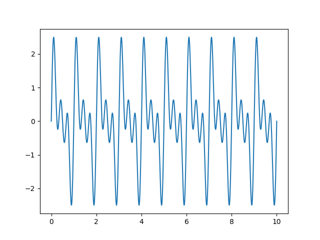
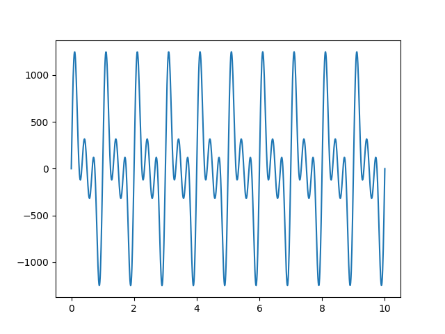
我们先制造一个信号
import matplotlib.pyplot as plt
import numpy as np


def create_signal(frequency, time: np.array):
    sin0 = np.sin(2 * np.pi * (frequency * time))
    sin1 = np.sin(2 * np.pi * (2 * frequency * time))
    sin2 = np.sin(2 * np.pi * (3 * frequency * time))

    return sin0 + sin1 + sin2

if "__main__" == __name__:
    time = np.linspace(0, 10, 1000)
    signal = create_signal(1, time=time)
    plt.plot(time, signal)

    plt.show()
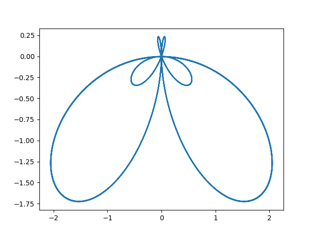
然后再制造出 e − i 2 π f t e^{-i2 \pi ft} e−i2πft 这个信号,让这两个信号相乘。注意这里 e − i 2 π f t e^{-i2 \pi ft} e−i2πft 信号的频率被设置为基频,相乘的结果如下:
import matplotlib.pyplot as plt
import numpy as np


def create_signal(frequency, time: np.array):
    sin0 = np.sin(2 * np.pi * (frequency * time))
    sin1 = np.sin(2 * np.pi * (2 * frequency * time))
    sin2 = np.sin(2 * np.pi * (3 * frequency * time))

    return sin0 + sin1 + sin2


def calculate_center_of_gravity(multi_signal):
    x_center = np.mean([x.real for x in multi_signal])
    y_center = np.mean([x.imag for x in multi_signal])

    return x_center, y_center


def calculate_sum(multi_signal):
    x_sum = np.sum([x.real for x in multi_signal])
    y_sum = np.sum([x.imag for x in multi_signal])

    return x_sum, y_sum


def create_pure_tone(frequency, time: np.array):
    angle = 2 * np.pi * frequency * time

    return np.cos(angle) - complex(0, 1) * np.sin(angle)


def plot_fourier_transform(signal,
                           pure_tone,
                           plot_center_of_gravity=False,
                           plot_sum=False):
    multi_signal = signal * pure_tone
    x_series = np.array([x.real for x in multi_signal])
    y_series = np.array([x.imag for x in multi_signal])

    plt.plot(x_series, y_series)

    if plot_center_of_gravity:
        center_of_gravity = calculate_center_of_gravity(multi_signal)
        plt.plot([center_of_gravity[0]], [center_of_gravity[1]],
                 marker='o',
                 markersize=10,
                 color="red")

    if plot_sum:
        integration = calculate_sum(multi_signal)
        plt.plot([integration[0]], [integration[1]],
                 marker='o',
                 markersize=10,
                 color="green")

    plt.show()


if "__main__" == __name__:
    time = np.linspace(0, 10, 1000)
    signal = create_signal(1, time=time)
    pure_tone = create_pure_tone(1, time=time)
    # plt.plot(time, pure_tone)

    # plt.show()

    plot_fourier_transform(signal,
                           pure_tone,
                           plot_center_of_gravity=False,
                           plot_sum=False)
好像不是很能看出问题,如果设置 e − i 2 π f t e^{-i2 \pi ft} e−i2πft 信号的频率为1.1呢,如下:

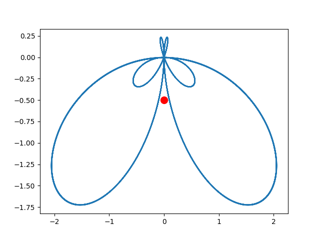
发现是对称图形,而此时如果求积分,且表示在图上,可得:
if "__main__" == __name__:
    time = np.linspace(0, 10, 1000)
    signal = create_signal(1, time=time)
    pure_tone = create_pure_tone(1.1, time=time)
    # plt.plot(time, pure_tone)

    # plt.show()

    plot_fourier_transform(signal,
                           pure_tone,
                           plot_center_of_gravity=True,
                           plot_sum=True)
其中 sum 是积分值,center_of_gravity 则是积分值除以采样点的个数,它们都在图中重合了,且积分值为0,所以1.1频率的 e − i 2 π f t e^{-i2 \pi ft} e−i2πft 信号与原始信号相似度很低。
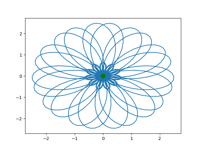
当 e − i 2 π f t e^{-i2 \pi ft} e−i2πft 信号的频率设置为1时,可得:
if "__main__" == __name__:
    time = np.linspace(0, 10, 1000)
    signal = create_signal(1, time=time)
    pure_tone = create_pure_tone(1.1, time=time)
    # plt.plot(time, pure_tone)

    # plt.show()

    plot_fourier_transform(signal,
                           pure_tone,
                           plot_center_of_gravity=True,
                           plot_sum=False)
在这里没有把积分值直接放上去,因为值太大了,但是 center_of_gravity 其实就是将 sum 除以采样点的个数,因此可以一定程度上代表 sum。
center_of_gravity 就是 g ^ ( f ) \hat{g}(f) g^(f) 的运算结果的实部和虚部,都除以采样点的个数,所以不影响辐角,其辐角为 − π 2 - \frac{\pi }{2} −2π,这个辐角对于 e − i 2 π f t e^{-i2 \pi ft} e−i2πft 信号的频率设置为2或3时,都是一样的:


接下来求出当 e − i 2 π f t e^{-i2 \pi ft} e−i2πft 信号的频率设置为1、2、3时,对应的 c 1 , c 2 , c 3 c_1, c_2, c_3 c1,c2,c3:
c 1 = 0 − j 499.5 c 2 = 0 − j 499.5 c 3 = 0 − j 499.5 \begin{aligned} c_1 = 0-j499.5 \\ c_2 = 0-j499.5 \\ c_3 = 0-j499.5 \end{aligned} c1=0−j499.5c2=0−j499.5c3=0−j499.5
傅里叶逆变换
傅里叶逆变换的公式可以直接给出:
f ( t ) = ∫ c f ⋅ e i 2 π f t d f f(t) = \int c_f \cdot e^{i2 \pi ft} df f(t)=∫cf⋅ei2πftdf
从这个形式上看,本质上就是用复数,对不同频率的 e i 2 π f t e^{i2 \pi ft} ei2πft 信号进行加权求。
傅里叶逆变换的代码与效果如下,注意是对 e i 2 π f t e^{i2 \pi ft} ei2πft 信号进行加权求和,可以对 e − i 2 π f t e^{-i2 \pi ft} e−i2πft 信号取共轭复数得到:
import matplotlib.pyplot as plt
import numpy as np


def create_signal(frequency, time: np.ndarray):
    sin0 = np.sin(2 * np.pi * (frequency * time))
    sin1 = np.sin(2 * np.pi * (2 * frequency * time))
    sin2 = np.sin(2 * np.pi * (3 * frequency * time))

    return sin0 + sin1 + sin2


def create_pure_tone(frequency, time: np.ndarray):
    angle = 2 * np.pi * frequency * time

    return np.cos(angle) - complex(0, 1) * np.sin(angle)


def calculate_mean(multi_signal):
    x_mean = np.mean([x.real for x in multi_signal])
    y_mean = np.mean([x.imag for x in multi_signal])

    return x_mean, y_mean


def calculate_sum(multi_signal):
    x_sum = np.sum([x.real for x in multi_signal])
    y_sum = np.sum([x.imag for x in multi_signal])

    return x_sum, y_sum


def plot_fourier_transform(signal,
                           pure_tone,
                           plot_mean=False,
                           plot_sum=False,
                           plot=True):
    multi_signal = signal * pure_tone
    x_series = np.array([x.real for x in multi_signal])
    y_series = np.array([x.imag for x in multi_signal])

    mean = calculate_mean(multi_signal)
    sum = calculate_sum(multi_signal)

    if plot:
        plt.plot(x_series, y_series)
        if plot_mean:
            plt.plot([mean[0]], [mean[1]],
                     marker='o',
                     markersize=10,
                     color="red")
        if plot_sum:
            plt.plot([sum[0]], [sum[1]],
                     marker='o',
                     markersize=10,
                     color="green")
        plt.show()

    return complex(mean[0], mean[1]), complex(sum[0], sum[1])


def plot_inverse_fourier_transform(cfs, pure_tones, time, plot=True):
    assert len(cfs) == len(pure_tones)
    signal = 0
    for i in range(len(cfs)):
        signal += cfs[i] * np.conj(pure_tones[i])

    if plot:
        plt.plot(time, signal)
        plt.show()

    return signal


if "__main__" == __name__:
    time = np.linspace(0, 10, 1000)
    signal = create_signal(frequency=1, time=time)
    pure_tone0 = create_pure_tone(frequency=1, time=time)
    pure_tone1 = create_pure_tone(frequency=2, time=time)
    pure_tone2 = create_pure_tone(frequency=3, time=time)

    pure_tones = [pure_tone0, pure_tone1, pure_tone2]
    cfs = []
    for pure_tone in pure_tones:
        mean, sum = plot_fourier_transform(signal,
                                           pure_tone,
                                           plot_mean=True,
                                           plot_sum=True,
                                           plot=False)
        cfs.append(sum)

    plot_inverse_fourier_transform(cfs, pure_tones, time)
可见其波形与原始信号已经非常相似,但是我们也看出一个明显的问题:为什么幅值比原始信号大了那么多?!
下一部分将与离散傅里叶变换有关,希望能够解释上面的问题。