前情提要
傅里叶变换的公式:
F ^ ( f ) = ∫ f ( t ) e − i 2 π f t d t \hat{F}(f) = \int f(t) e^{-i2 \pi ft} dt F^(f)=∫f(t)e−i2πftdt
傅里叶逆变换的公式:
f ( t ) = ∫ F ^ ( f ) e i 2 π f t d f f(t) = \int \hat{F}(f) e^{i2 \pi ft} df f(t)=∫F^(f)ei2πftdf
之前我们遇到的问题是:直接用傅里叶逆变换的公式得到的重建信号,幅值要远远大于原始信号。
- 重建信号
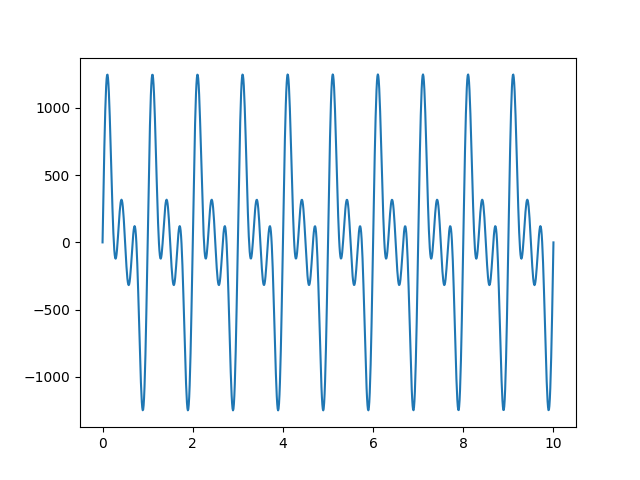
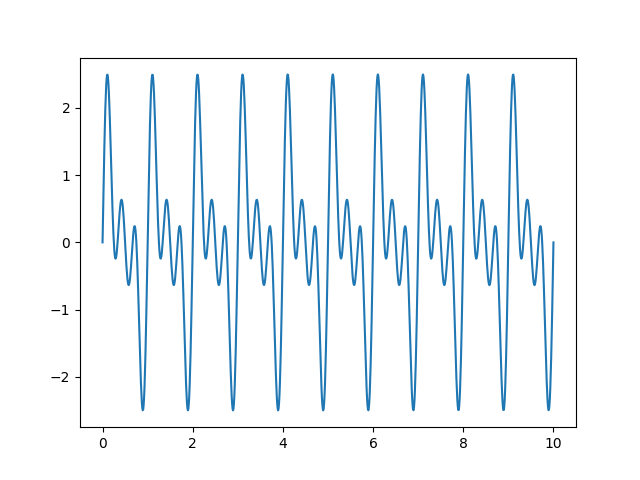
- 原始信号
现在可以告诉大家原因:用计算机做的傅里叶变换本质上是离散傅里叶变换,因此要重建信号,也应该用离散傅里叶逆变换。
离散傅里叶变换
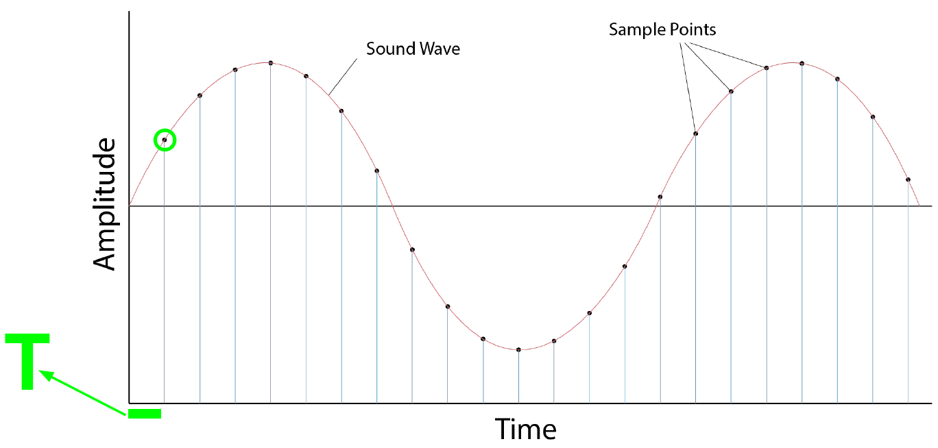
傅里叶变换的公式 F ^ ( f ) = ∫ f ( t ) e − i 2 π f t d t \hat{F}(f) = \int f(t) e^{-i2 \pi ft} dt F^(f)=∫f(t)e−i2πftdt 中的 f ( t ) f(t) f(t) 表示连续的时序信号,在计算机中会被离散化,即:采样->量化->编码。下图中的T为采样周期,即计算机中每个采样点的间隔时间,数字化之后 f ( t ) f(t) f(t) 会变成 x ( n ) x(n) x(n), x ( n ) = f ( n T ) x(n)=f(nT) x(n)=f(nT)。
接下来一步一步将傅里叶变换的公式也离散化:
- 公式中的信号的符号要变成离散的形式,并且积分符号要变成求和符号
X ^ ( f ) = ∑ n x ( n ) e − i 2 π f n \hat{X} (f) = \sum_{n} x(n) e^{-i2 \pi fn} X^(f)=n∑x(n)e−i2πfn
于是,原始信号和 e − i 2 π f n e^{-i2 \pi fn} e−i2πfn 信号都变成了离散形式,变成了可以用下边n访问的一个数组。 - 还有两个问题:
- 原始信号在时序上是无穷的,如何在计算机中表示原始信号?
- 需要选择不同频率的 e − i 2 π f n e^{-i2 \pi fn} e−i2πfn 信号,找出对应的最佳振幅和初相,而这些可能的频率也是无穷多个的,如何在计算机中得到这些不同频率的 e − i 2 π f n e^{-i2 \pi fn} e−i2πfn 信号呢?
- 办法还是有的:
- 假设需要分解的原始信号的频率在一段有限时序区间内是非零的。这个好理解,一首3分钟的歌曲应该已经具有足够的信息,用于频率分解。
X ^ ( f ) = ∑ n = 0 N − 1 x ( n ) e − i 2 π f n \hat{X} (f) = \sum_{n=0}^{N-1} x(n) e^{-i2 \pi fn} X^(f)=n=0∑N−1x(n)e−i2πfn - 只选取有限个频率,得到有限个 e − i 2 π f n e^{-i2 \pi fn} e−i2πfn 信号,对这些有限个信号,找寻最佳的振幅和初相。
- 所选取的有限个频率的数量,最好与原始信号在一段有限时序区间内的采样点的个数相同,这样做主要是为了能够较好的进行傅里叶逆变换。
X ^ ( k N ) = ∑ n = 0 N − 1 x ( n ) e − i 2 π k N n , k = 0 , 1 , 2 , . . . , N − 1 \hat{X} (\frac{k}{N}) = \sum_{n=0}^{N-1} x(n) e^{-i2 \pi \frac{k}{N}n},k=0,1,2,...,N-1 X^(Nk)=n=0∑N−1x(n)e−i2πNkn,k=0,1,2,...,N−1 - k的实际含义是什么呢?为何 k N \frac{k}{N} Nk 能够取代频率f的位置呢?实际上k与f之间存在映射关系,函数表示为:
f = g ( k ) = k N T = k ⋅ s r N f = g(k) = \frac{k}{NT} =\frac{k \cdot s_r}{N} f=g(k)=NTk=Nk⋅sr
其中sr为原始信号的采样频率。也就是说,所选取的频率范围是[0, sr),在这范围内,以采样点的个数等分选取频率。
- 假设需要分解的原始信号的频率在一段有限时序区间内是非零的。这个好理解,一首3分钟的歌曲应该已经具有足够的信息,用于频率分解。
离散傅里叶逆变换
离散傅里叶逆变换的公式可以直接给出:
x ( n ) = 1 N ∑ k = 0 N − 1 X ^ ( k N ) e i 2 π k N n x(n) = \frac{1}{N} \sum_{k=0}^{N-1} \hat{X} (\frac{k}{N}) e^{i2 \pi \frac{k}{N}n} x(n)=N1k=0∑N−1X^(Nk)ei2πNkn
import matplotlib.pyplot as plt
import numpy as np


def create_signal(frequency, time: np.ndarray):
    sin0 = np.sin(2 * np.pi * (frequency * time))
    sin1 = np.sin(2 * np.pi * (2 * frequency * time))
    sin2 = np.sin(2 * np.pi * (3 * frequency * time))

    return sin0 + sin1 + sin2


def create_pure_tone(frequency, time: np.ndarray):
    angle = 2 * np.pi * frequency * time

    return np.cos(angle) - complex(0, 1) * np.sin(angle)


def calculate_mean(multi_signal):
    x_mean = np.mean([x.real for x in multi_signal])
    y_mean = np.mean([x.imag for x in multi_signal])

    return x_mean, y_mean


def calculate_sum(multi_signal):
    x_sum = np.sum([x.real for x in multi_signal])
    y_sum = np.sum([x.imag for x in multi_signal])

    return x_sum, y_sum


def plot_fourier_transform(signal,
                           pure_tone,
                           plot_mean=False,
                           plot_sum=False,
                           plot=True):
    multi_signal = signal * pure_tone
    x_series = np.array([x.real for x in multi_signal])
    y_series = np.array([x.imag for x in multi_signal])

    mean = calculate_mean(multi_signal)
    sum = calculate_sum(multi_signal)
    # print(f"mean:{mean}\nsum:{sum}")

    if plot:
        plt.plot(x_series, y_series)
        if plot_mean:
            plt.plot([mean[0]], [mean[1]],
                     marker='o',
                     markersize=10,
                     color="red")
        if plot_sum:
            plt.plot([sum[0]], [sum[1]],
                     marker='o',
                     markersize=10,
                     color="green")
        plt.show()

    return complex(mean[0], mean[1]), complex(sum[0], sum[1])


def plot_inverse_fourier_transform(cfs, pure_tones, time, plot=True):
    assert len(cfs) == len(pure_tones)
    N = len(cfs)
    signal = 0
    for i in range(N):
        signal += cfs[i] * np.conj(pure_tones[i])
    signal /= N

    if plot:
        plt.plot(time, signal)
        plt.show()

    return signal


if "__main__" == __name__:
    time = np.linspace(0, 10, 1000)
    N = time.shape[0]
    sr = 1000 // (10 - 0)

    signal = create_signal(frequency=1, time=time)

    pure_tones = []
    for k in np.linspace(0, N, N, endpoint=False):
        pure_tone = create_pure_tone(frequency=k * sr / N, time=time)
        pure_tones.append(pure_tone)

    cfs = []
    for pure_tone in pure_tones:
        mean, sum = plot_fourier_transform(signal,
                                           pure_tone,
                                           plot_mean=True,
                                           plot_sum=True,
                                           plot=False)
        cfs.append(sum)

    rebuild = plot_inverse_fourier_transform(cfs, pure_tones, time, plot=False)

    plt.plot(time, signal, label="signal")
    plt.plot(time, rebuild, label="rebuild")
    plt.fill_between(time, signal * rebuild, alpha=0.25)
    plt.legend()

    plt.show()

    # np.testing.assert_array_almost_equal(signal, rebuild)
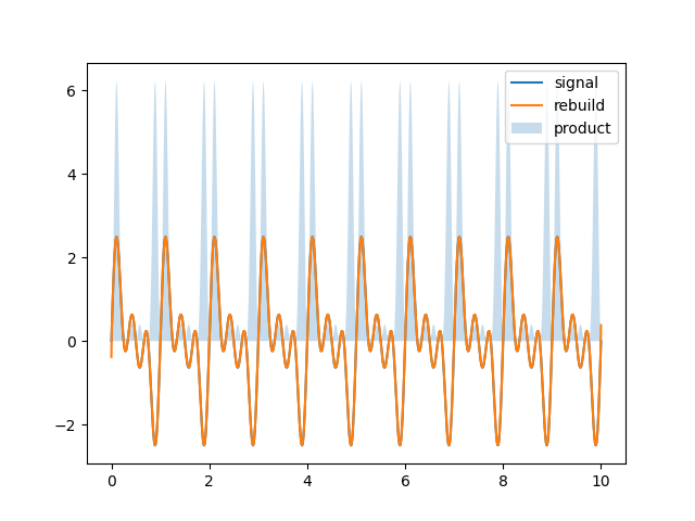
原始信号与重建信号几乎重合,且乘积也全部为正数!
可以用numpy的单元测试,逐点计算一下误差:
np.testing.assert_array_almost_equal(signal, rebuild)
Arrays are not almost equal to 6 decimals

Mismatched elements: 996 / 1000 (99.6%)
Max absolute difference: 0.00249961
Max relative difference: 1.05935375
 x: array([ 0.000000e+00,  3.758780e-01,  7.428670e-01,  1.092347e+00,
        1.416225e+00,  1.707181e+00,  1.958881e+00,  2.166163e+00,
        2.325182e+00,  2.433514e+00,  2.490210e+00,  2.495807e+00,...
 y: array([ 8.928912e-14-8.203696e-14j,  3.755021e-01-1.757345e-13j,
        7.421241e-01-8.970006e-14j,  1.091254e+00-9.888207e-14j,
        1.414809e+00-5.689618e-15j,  1.705474e+00-3.955452e-15j,...
最大相对误差为1.05935375%。
与numpy比较
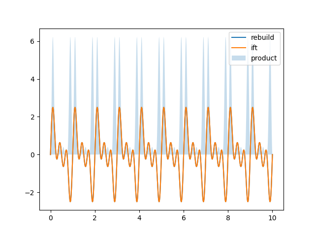
numpy的fft效果极佳,尽管自己写的rebuild与ift波形重合,但ift绝对误差小于小数点后14位。
    # numpy
    ft = np.fft.fft(signal)
    ift = np.fft.ifft(ft)
    plt.plot(time, rebuild, label="rebuild")
    plt.plot(time, ift, label="ift")
    plt.fill_between(time, rebuild * ift, alpha=0.25, label="product")
    plt.legend()

    plt.show()

    np.testing.assert_array_almost_equal(signal, ift, decimal=20)
Arrays are not almost equal to 20 decimals

Mismatched elements: 1000 / 1000 (100%)
Max absolute difference: 1.875756e-15
Max relative difference: 1.
 x: array([ 0.0000000000000000e+00,  3.7587797360061515e-01,
        7.4286697945743752e-01,  1.0923466914234694e+00,
        1.4162251787527200e+00,  1.7071811899304179e+00,...
 y: array([ 0.0000000000000000e+00-9.2967300524549044e-17j,
        3.7587797360061515e-01-7.7896022965262552e-17j,
        7.4286697945743785e-01+1.0284828544371295e-16j,...
fft的算法复杂度是 O ( N ⋅ l o g 2 N ) O(N \cdot log_2 N) O(N⋅log2N),只有当采样点数为2的整数次幂时才能运行。
对称性
记得在深入理解傅里叶变换(一)中提到:将选择的频率作为横坐标,对应的波的振幅作为纵坐标,会得到被称为频谱图(spectrum)的东西,如下图所示:
if "__main__" == __name__:
    time = np.linspace(0, 10, 1000)
    sr = 1000 // (10 - 0)
    signal = create_signal(frequency=1, time=time)
    N = signal.size

    pure_tones = []
    frequencies = []
    for k in np.linspace(0, N, N, endpoint=False):
        pure_tone = create_pure_tone(frequency=k * sr / N, time=time)
        pure_tones.append(pure_tone)
        frequencies.append(k * sr / N)

    cfs = []
    for pure_tone in pure_tones:
        mean, sum = plot_fourier_transform(signal,
                                           pure_tone,
                                           plot_mean=True,
                                           plot_sum=True,
                                           plot=False)
        cfs.append(sum)
        print(len(cfs))

    magnitudes = np.abs(cfs)
    rebuild = plot_inverse_fourier_transform(cfs, pure_tones, time, plot=False)
    plt.plot(frequencies, magnitudes, label="spectrum")

    plt.legend()
    plt.show()
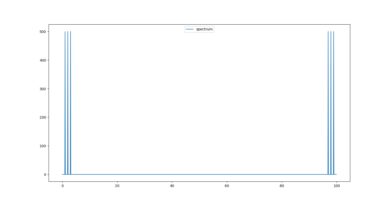
发现这图是左右对称的,中心是 s r 2 \frac{s_r}{2} 2sr。
原因是:对于一个周期信号而言,如果想要准确地度量这个信号,则需要在每个周期进行至少两次采样 : 对波峰部分采样一次 , 对波谷部分采样一次。每个周期的采样越多 ,越能准确地重建原始信号。但是,如果在每个周期的采样不足两次,那么将完全丢失原始信号的频率信息,也不可能重建原始信号 。
现在我们对原始信号的采样率是 s r s_r sr,那么可知这个采样率最多让我们重建原始信号中蕴含的最高频率为 s r 2 \frac{s_r}{2} 2sr 的信号,更高频的信号不可能重建出来。
定理:给定一个采样率,我们所能重建的周期信号的频率是该采样率的一半。该采样率的一半被称为奈奎斯特频率,也就是上图的中心 s r 2 \frac{s_r}{2} 2sr。
下一节讲短时傅里叶变换。