时间序列分析之GARCH模型介绍与应用
前言
RNN(循环神经网络)是一种节点定向连接成环的人工神经网络。不同于前馈神经网络,RNN可以利用内部的记忆来处理任意时序的输入序列,即不仅学习当前时刻的信息,也会依赖之前的序列信息,所以在做语音识别、语言翻译等等有很大的优势。RNN现在变种很多,常用的如LSTM、Seq2SeqLSTM,还有其他变种如含有Attention机制的Transformer模型等等。这些变种原理结构看似很复杂,但其实只要有一定的数学和计算机功底,在学习的时候认认真真搞懂一个,后面的都迎刃而解。
本文将对LSTM里面知识做高度浓缩介绍(包括前馈推导和链式法则),然后再建立时序模型和优化模型,最后评估模型并与ARIMA或ARIMA-GARCH模型做对比!
一:RNN神经网络底层逻辑介绍
(注:下面涉及的所有模型解释图来源于百度图片)
- 输入层、隐藏层和输出层
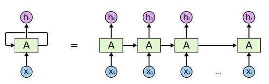
从上图1,假设 X t ∈ R n × x X_t\in R^{n\times x} Xt∈Rn×x 是序列中第 t t t 个批量输入(这里的 n n n 是样本个数, x x x 是样本特征维度),对应隐藏层状态为 h t ∈ R n ∗ h h_t\in R^{n * h} ht∈Rn∗h ( h h h 为隐藏层长度),最终输出 Y t = R n ∗ y Y_t = R^{n*y} Yt=Rn∗y ( y y y 为输出向量维度,即输出向量到底含几个元素!)。那么在计算 t t t 时刻 h h h ,有公式:
h t = ϕ ( X t W x h + h t − 1 W n h + b h ) h_t=\phi(X_tW_{xh}+h_{t-1}W_{nh}+b_h) ht=ϕ(XtWxh+ht−1Wnh+bh) ,
这里的 ϕ \phi ϕ 为某一特定激活函数, W . , . W_{.,.} W.,. 为需要学习的权重, b . b_. b. 为要学习的偏差值,那么同理输出结果为:
o t = ϕ ( h t W y h + b y ) o_t=\phi(h_tW_{yh}+b_y) ot=ϕ(htWyh+by) ,参数解释如上!
- 损失函数定义
根据误差函数性质,对于回归问题,大多数建立的是基于距离形式的均方误差函数或者绝对误差函数,如果是分类问题,我们一般会选择交叉熵这类函数!
t t t 时刻有误差 l t = Δ ( Y t , o t ) l_t=\Delta(Y_t,o_t) lt=Δ(Yt,ot) ,这里的 Y t Y_t Yt 为真实值, o t o_t ot 为预测值。那么整个时间长度 T T T ,我们有
L = 1 T ∑ t = 1 T l t ( Y t , o t ) L=\frac{1}{T}\sum_{t=1}^{T}{l_t(Y_t,o_t)} L=T1∑t=1Tlt(Yt,ot) ,
我们的目的就是更新所有的参数 W . , . W_.,. W.,. 和 b . b_. b. 使 L L L 最小。
- 梯度下降与链式法则求导
这里的推导比较复杂,为了让大家能理解到整个模型思想而不是存粹学术研究,只做重点介绍!且激活函数简化!
对于参数 W . , . W_{.,.} W.,. 的更新,经典的梯度下降格式为: W . , . = W . , . − η ∂ L ∂ W . , . W_{.,.}=W_{.,.}-\eta\frac{\partial L}{\partial W_{.,.}} W.,.=W.,.−η∂W.,.∂L ,根据微积分知识,我们知道链式法则公式为:若 Y = f ( X ) , Z = g ( Y ) Y=f(X),Z=g(Y) Y=f(X),Z=g(Y) ,那么
∂ Z ∂ X = p r o d ( ∂ Z ∂ Y , ∂ Y ∂ X ) \frac{\partial Z}{\partial X}=prod(\frac{\partial Z}{\partial Y},\frac{\partial Y}{\partial X}) ∂X∂Z=prod(∂Y∂Z,∂X∂Y) 可以表示为链式求导过程!
现在开始推导各个函数的链式求导结果,对于任意 t t t 时刻的输出 o t o_t ot ,由损失函数定义很容易知:
∂ L ∂ o t = 1 T ∂ L ( y t , o t ) ∂ o t \frac{\partial L}{\partial o_t}=\frac{1}{T}\frac{\partial L(y_t,o_t)}{\partial o_t} ∂ot∂L=T1∂ot∂L(yt,ot) ,
那么对于 W y h W_{yh} Wyh 的更新,由 T T T步才能到 L L L ,求和可得:
∂ L ∂ W y h = p r o d ( ∂ L ∂ o t , ∂ o t ∂ W y h ) = ∑ t = 1 T ∂ L ∂ o t h t T \frac{\partial L}{\partial W_{yh}}={prod(\frac{\partial L}{\partial o_t},\frac{\partial o_t}{\partial W_{yh}})}=\sum_{t=1}^{T}{\frac{\partial L}{\partial o_t}h_t^{T}} ∂Wyh∂L=prod(∂ot∂L,∂Wyh∂ot)=∑t=1T∂ot∂LhtT ,
对于终端时刻 T T T ,我们很容易有:
∂ L ∂ h T = p r o d ( ∂ L ∂ o T , ∂ o T ∂ h T ) = W y h T ∂ L ∂ o T \frac{\partial L}{\partial h_T}=prod(\frac{\partial L}{\partial o_T},\frac{\partial o_T}{\partial h_T})=W_{yh}^T\frac{\partial L}{\partial o_T} ∂hT∂L=prod(∂oT∂L,∂hT∂oT)=WyhT∂oT∂L ,
但对于 t < T t<T t<T 时刻而言,对于隐藏层的求导比较复杂,因为有个时间前后关系,所以我们有:
∂ L ∂ h t = p r o d ( ∂ L ∂ h t + 1 , ∂ h t + 1 ∂ h t ) + p r o d ( ∂ L ∂ o t , ∂ o t ∂ h t ) = W n h T ∂ L ∂ h t + 1 + W y h T ∂ L ∂ o t ( ∗ ) \frac{\partial L}{\partial h_t}=prod(\frac{\partial L}{\partial h_{t+1}},\frac{\partial h_{t+1}}{\partial h_t})+prod(\frac{\partial L}{\partial o_t},\frac{\partial o_t}{\partial h_t})=W_{nh}^T\frac{\partial L}{\partial h_{t+1}}+W_{yh}^T\frac{\partial L}{\partial o_t}(*) ∂ht∂L=prod(∂ht+1∂L,∂ht∂ht+1)+prod(∂ot∂L,∂ht∂ot)=WnhT∂ht+1∂L+WyhT∂ot∂L(∗)
那么同理,很容易我们将解决:
∂ L ∂ W x h = p r o d ( ∂ L ∂ h t , ∂ h t ∂ W x h ) = ∑ t = 1 T ∂ L ∂ h t x t T \frac{\partial L}{\partial W_{xh}}=prod(\frac{\partial L}{\partial h_t},\frac{\partial h_t}{\partial W_{xh}})=\sum_{t=1}^{T}{\frac{\partial L}{\partial h_t}}x_t^T ∂Wxh∂L=prod(∂ht∂L,∂Wxh∂ht)=∑t=1T∂ht∂LxtT
以及 ∂ L ∂ W n h = p r o d ( ∂ L ∂ h t , ∂ h t ∂ W n h ) = ∑ t = 1 T ∂ L ∂ h t h t − 1 T \frac{\partial L}{\partial W_{nh}}=prod(\frac{\partial L}{\partial h_t},\frac{\partial h_t}{\partial W_{nh}})=\sum_{t=1}^{T}{\frac{\partial L}{\partial h_t}h_{t-1}^T} ∂Wnh∂L=prod(∂ht∂L,∂Wnh∂ht)=∑t=1T∂ht∂Lht−1T
二:对于梯度消散(爆炸)的原理解释
一般RNN模型,会因为在链式法则中存在梯度消散(爆炸)的问题,所以我们要发展新的变种来解决这种问题,那么这梯度问题到底在哪呢?仔细发现在上一节的 ( ∗ ) (*) (∗)式推导过程中,对于隐藏层求导,我们继续对 ( ∗ ) (*) (∗)式改写可得:
∂ L ∂ h t + 1 = p r o d ( ∂ L ∂ h t + 2 , ∂ h t + 2 ∂ h t + 1 ) + p r o d ( ∂ L ∂ o t + 1 , ∂ o t + 1 ∂ h t + 1 ) \frac{\partial L}{\partial h_{t+1}}=prod(\frac{\partial L}{\partial h_{t+2}},\frac{\partial h_{t+2}}{\partial h_{t+1}})+prod(\frac{\partial L}{\partial o_{t+1}},\frac{\partial o_{t+1}}{\partial h_{t+1}}) ∂ht+1∂L=prod(∂ht+2∂L,∂ht+1∂ht+2)+prod(∂ot+1∂L,∂ht+1∂ot+1)
= W n h T ∂ L ∂ h t + 2 + W y h T ∂ L ∂ o t + 1 ( ∗ ∗ ) =W_{nh}^T\frac{\partial L}{\partial h_{t+2}}+W_{yh}^T\frac{\partial L}{\partial o_{t+1}}(**) =WnhT∂ht+2∂L+WyhT∂ot+1∂L(∗∗) ,
我们再对 ( ∗ ∗ ) (**) (∗∗) 往后推一步,然后依次推到 T 时刻,最终由数学归纳法易得到:
∂ L ∂ h t = ∑ i = 1 T ( W n h T ) T − i W y h T ∂ L ∂ o T + t − i \frac{\partial L}{\partial h_t}=\sum_{i=1}^{T}{(W_{nh}^T)^{T-i}W_{yh}^T\frac{\partial L}{\partial o_{T+t-i}}} ∂ht∂L=∑i=1T(WnhT)T−iWyhT∂oT+t−i∂L ,
由此式我们知道当 T 、 t T、t T、t 变大或变小,对于幂次计算,结果会突变大或者趋于平稳消散不见!由此一般RNN理论介绍到此,想具体了解的可以查阅相关论文。
三:LSTM底层理论介绍
为了更好的捕获时序中间隔较大的依赖关系,基于门控制的长短记忆网络(LSTM)诞生了!
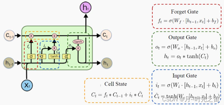
所谓“门”结构就是用来去除或者增加信息到细胞状态的能力。这里的细胞状态是核心,它属于隐藏层,类似于传送带,在整个链上运行,信息在上面流传保持不变会变得很容易!
上图2非常形象生动描绘了LSTM核心的“三门结构”。红色圈就是所谓的遗忘门,那么在 t 时刻如下公式表示(如果我们真理解了RNN逻辑,LSTM理解起来将变得比较轻松):
F t = ϕ ( X t W x f + h t − 1 W h f + b f ) F_t=\phi(X_tW_{xf}+h_{t-1}W_{hf}+b_f) Ft=ϕ(XtWxf+ht−1Whf+bf) ,
蓝圈输入门有 I t = ϕ ( X t W x i + h t − 1 W h i + b i ) I_t=\phi(X_tW_{xi}+h_{t-1}W_{hi}+b_i) It=ϕ(XtWxi+ht−1Whi+bi) ,
绿圈输出门有 o t = ϕ ( X t W x o + h t − 1 W h o + b o ) o_t=\phi(X_tW_{xo}+h_{t-1}W_{ho}+b_o) ot=ϕ(XtWxo+ht−1Who+bo) ,
同理以上涉及的参数 W . , . W_{.,.} W.,. 和 b . b_. b. 为需要通过链式法则更新的参数!那么最后黄圈的细胞信息计算公式:
C t = F t ∗ C t − 1 + I t ∗ C t ˉ C_t=F_t\ast C_{t-1}+I_t\ast \bar{C_t} Ct=Ft∗Ct−1+It∗Ctˉ ,其中
C t ˉ = t a n h ( X t W x c + h t − 1 W h c + b c ) \bar{C_t}=tanh(X_tW_{xc}+h_{t-1}W_{hc}+b_c) Ctˉ=tanh(XtWxc+ht−1Whc+bc) ,
这里涉及的双曲正切函数 t a n h ∈ [ − 1 , 1 ] tanh\in [-1,1] tanh∈[−1,1] 一般是固定的,那么费这么大事,搞这么多信息控制过程是为了什么?当然是为了更新细胞 C t C_t Ct 值从而为了获取下一步隐藏层的值: h t = o t ∗ t a n h ( C t ) h_t=o_t*tanh(C_t) ht=ot∗tanh(Ct) 。
当 ϕ \phi ϕ 激活函数选择 s i g m o i d sigmoid sigmoid属于 0 1 0~1 0 1的函数时,对于遗忘门近似等于1,输入门近似等于0,其实 C t C_t Ct 是不更新的,那么过去的细胞信息一直保留到现在,解决了梯度消散问题。
同理,输出门可以近似等于1,也可以近似等于0,那么近似等于1时细胞信息将传递给隐藏层;近似等于0时,细胞信息只自己保留。至此所有参数更新一遍并继续向下走。。。
PS:也许初学者看到这么多符号会比较头疼,但逻辑是从简到复杂的,RNN彻底理解有助于理解后面的深入模型。这里本人也省略了很多细节,大体模型框架就是如此,对于理解模型如何工作已经完全够了。至于怎么想出来的以及更为详细的推导过程,由于作者水平有限,可参考相关RNN论文,可多交流学习!
四:建模预测存在“右偏移”怎么办!
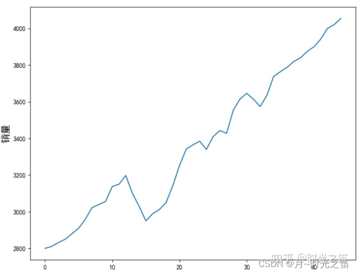
为了做对比实验,我们还会选择之前时序文章所对应的实际销量数据!我们将基于keras模块构建自己的LSTM网络进行时序预测。
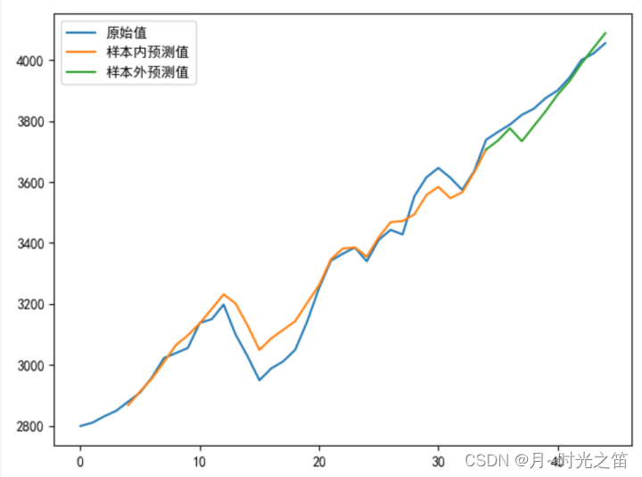
- 构建一般LSTM模型,当我们选择步长为1时,先给出结果如下
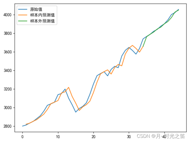
正常建立LSTM模型预测会出现如上预测值右偏现象,尽管r2或者MSE很好,但这建立的模型其实是无效模型!
- 原因与改进
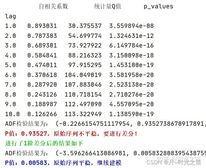
当模型倾向于把上一时刻的真实值作为下一时刻的预测值,导致两条曲线存在滞后性,也就是真实值曲线滞后于预测值曲线,如图4那样。之所以会这样,是因为序列存在自相关性,如一阶自相关指的是当前时刻的值与其自身前一时刻值之间的相关性。因此,如果一个序列存在一阶自相关,模型学到的就是一阶相关性。而消除自相关性的办法就是进行差分运算,也就是我们可以将当前时刻与前一时刻的差值作为我们的回归目标。
而且从之前文章做的白噪声检验也发现,该序列确实存在很强的自相关性!如下图5所示。
五:改进模型输出
我们看下模型最终输出结果:

- 经典时序模型下的最优输出结果
https://blog.csdn.net/weixin_43577256/article/details/121787085
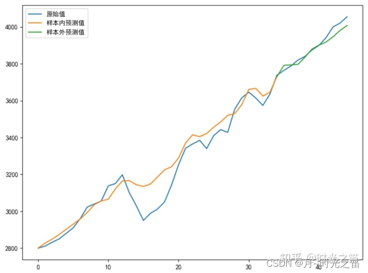

此结果的全局MSE=4401.02大于LSTM网络的MSE=2521.30,由此可见当我们优化LSTM模型后,一定程度上时序建模比ARIMA或者ARIMA-GARCH要优!
LSTM预测理论跟ARIMA也是有区别的,LSTM主要是基于窗口滑动取数据训练来预测滞后数据,其中的cell机制会由于权重共享原因减少一些参数;ARIMA模型是根据自回归理论,建立与自己过去有关的模型。两者共同点就是能很好运用序列数据,而且通过不停迭代能无限预测下去,但预测模型还是基于短期预测有效,长期预测必然会导致偏差很大,而且有可能出现预测值趋于不变的情况。
六:最终代码
from keras.callbacks import LearningRateScheduler
from sklearn.metrics import mean_squared_error
from keras.models import Sequential
import matplotlib.pyplot as plt
from keras.layers import Dense
from keras.layers import LSTM
from keras import optimizers
import keras.backend as K
import tensorflow as tf
import pandas as pd
import numpy as np

plt.rcParams['font.sans-serif']=['SimHei']##中文乱码问题!
plt.rcParams['axes.unicode_minus']=False#横坐标负号显示问题!

###初始化参数
my_seed = 369#随便给出个随机种子
tf.random.set_seed(my_seed)##运行tf才能真正固定随机种子

sell_data = np.array([2800,2811,2832,2850,2880,2910,2960,3023,3039,3056,3138,3150,3198,3100,3029,2950,2989,3012,3050,3142,3252,3342,3365,3385,3340,3410,3443,3428,3554,3615,3646,3614,3574,3635,3738,3764,3788,3820,3840,3875,3900,3942,4000,4021,4055])
num_steps = 3##取序列步长
test_len = 10##测试集数量长度
S_sell_data = pd.Series(sell_data).diff(1).dropna()##差分
revisedata = S_sell_data.max()
sell_datanormalization = S_sell_data / revisedata##数据规范化

##数据形状转换,很重要!!
def data_format(data, num_steps=3, test_len=5):
    # 根据test_len进行分组
    X = np.array([data[i: i + num_steps]
                  for i in range(len(data) - num_steps)])
    y = np.array([data[i + num_steps]
                  for i in range(len(data) - num_steps)])

    train_size = test_len
    train_X, test_X = X[:-train_size], X[-train_size:]
    train_y, test_y = y[:-train_size], y[-train_size:]
    return train_X, train_y, test_X, test_y

transformer_selldata = np.reshape(pd.Series(sell_datanormalization).values,(-1,1))
train_X, train_y, test_X, test_y = data_format(transformer_selldata, num_steps, test_len)
print('\033[1;38m原始序列维度信息:%s;转换后训练集X数据维度信息:%s,Y数据维度信息:%s;测试集X数据维度信息:%s,Y数据维度信息:%s\033[0m'%(transformer_selldata.shape, train_X.shape, train_y.shape, test_X.shape, test_y.shape))

def buildmylstm(initactivation='relu',ininlr=0.001):

    nb_lstm_outputs1 = 128#隐藏层1神经元个数
    nb_lstm_outputs2 = 128#隐藏层2神经元个数
    nb_time_steps = train_X.shape[1]#时间序列步长长度
    nb_input_vector = train_X.shape[2]#输入序列特征维度
    model = Sequential()
    model.add(LSTM(units=nb_lstm_outputs1, input_shape=(nb_time_steps, nb_input_vector),return_sequences=True))
    model.add(LSTM(units=nb_lstm_outputs2, input_shape=(nb_time_steps, nb_input_vector)))
    model.add(Dense(64, activation=initactivation))
    model.add(Dense(32, activation='relu'))
    model.add(Dense(test_y.shape[1], activation='tanh'))

    lr = ininlr
    adam = optimizers.adam_v2.Adam(learning_rate=lr)
    def scheduler(epoch):##编写学习率变化函数
        # 每隔epoch,学习率减小为原来的1/10
        if epoch % 100 == 0 and epoch != 0:
            lr = K.get_value(model.optimizer.lr)
            K.set_value(model.optimizer.lr, lr * 0.1)
            print('lr changed to {}'.format(lr * 0.1))
        return K.get_value(model.optimizer.lr)
    model.compile(loss='mse', optimizer=adam, metrics=['mse'])##根据损失函数性质,回归建模一般选用”距离误差“作为损失函数,分类一般选”交叉熵“损失函数
    reduce_lr = LearningRateScheduler(scheduler)
    ###数据集较少,全参与形式,epochs一般跟batch_size成正比
    ##callbacks:回调函数,调取reduce_lr
    ##verbose=0:非冗余打印,即不打印训练过程
    batchsize = int(len(sell_data) / 5)
    epochs = max(128,batchsize * 4)##最低循环次数128
    model.fit(train_X, train_y, batch_size=batchsize, epochs=epochs, verbose=0, callbacks=[reduce_lr])

    return model

def prediction(lstmmodel):

    predsinner = lstmmodel.predict(train_X)
    predsinner_true = predsinner * revisedata
    init_value1 = sell_data[num_steps - 1]##由于存在步长关系,这里起始是num_steps
    predsinner_true = predsinner_true.cumsum()  ##差分还原
    predsinner_true = init_value1 + predsinner_true

    predsouter = lstmmodel.predict(test_X)
    predsouter_true = predsouter * revisedata
    init_value2 = predsinner_true[-1]
    predsouter_true = predsouter_true.cumsum()  ##差分还原
    predsouter_true = init_value2 + predsouter_true

    # 作图
    plt.plot(sell_data, label='原始值')
    Xinner = [i for i in range(num_steps + 1, len(sell_data) - test_len)]
    plt.plot(Xinner, list(predsinner_true), label='样本内预测值')
    Xouter = [i for i in range(len(sell_data) - test_len - 1, len(sell_data))]
    plt.plot(Xouter, [init_value2] + list(predsouter_true), label='样本外预测值')
    allpredata = list(predsinner_true) + list(predsouter_true)
    plt.legend()
    plt.show()

    return allpredata

mymlstmmodel = buildmylstm()
presult = prediction(mymlstmmodel)

def evaluate_model(allpredata):

    allmse = mean_squared_error(sell_data[num_steps + 1:], allpredata)
    print('ALLMSE:',allmse)

evaluate_model(presult)
上述代码可直接复制使用,关键地方本人都有注释,如有不清楚地方可以多多交流,也许此模型还有优化地方,可多多交流。对于LSTM建模,数据维度转换是必要步骤,大家要认真理解!
七:总结
任何模型都不是万能的,重点是要有发现问题和解决问题的能力。
小数据建模往往比大数据要更难,更要思考。
对于深度模型学习,本人还是强烈建议要大致懂模型的内涵和原理,有条件甚至可以自己推导一遍或者简单实现下梯度下降算法、损失函数构建等等,否则很难解决真正的问题。
由于本人能力有限,有兴趣朋友者多多交流,点赞关注加收藏,再次表示感谢!