上篇提到的卷积神经网络对手写数字的识别,识别率为99.15%,作为对比,我们对比一下线性模型LN、单神经网络SN、深度神经网络DNN对相同的测试数据进行模拟,才能看到卷积神经网络的强大。
测试结果如下:
| 模型名称 | 正确率 |
|---|---|
| 卷积神经网络 | 99.15% |
| 线性模型 | 31.32% |
| 单神经元模型 | 92.49% |
| 深度神经网络 | 96.97% |
结论和分析:卷积神经网络在图像处理领域无人能敌。
| 模型名称 | 分析原因 |
|---|---|
| 线性模型 | 只能划分线性问题,非线性问题无能为力 |
| 单神经元模型 | 可以处理非线性问题,结构过于简单,对特征的提取力度不够 |
| 深度神经网络 | 可以提取非常多的特征,也正因为提取了所有细节,导致了过拟合,结果反而不好。太扣细节 |
| 卷积神经网络 | 可以理解为稀疏的深度神经网络。卷积、池化等的操作,实际上就是选择局部图片信息提取特征,从而降低了复杂度,也避免了过拟合,多个卷积核从多方面提取特征,构成的特征很全面,但又不是在意每个细节 |
用TensorFlow2实现各种模型
基于上篇的卷积神经网络,稍作更改,就能得到各种各样的模型。
一、线性模型
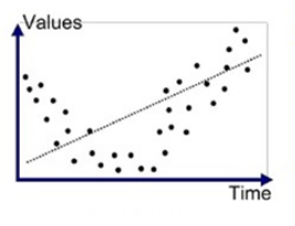
线性模型就是我们常说的 y = k*x + b 。只能表示线性的划分。模型如下:
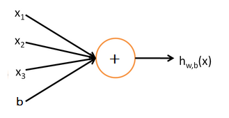
只能拟合这样的曲线:
tf实现方式:用一个全连接Dense,激活函数用线性函数。
代码如下:from testData import * 中的testData见上一篇文章。testData
import numpy as np
import tensorflow as tf
from testData import *
import time

class LINE(tf.keras.Model):
    def __init__(self):
        super().__init__()
        self.line = tf.keras.layers.Dense(units=10,activation=tf.keras.activations.linear)  #一个神经元的全连接网络,激活函数是线性的
        self.flatten = tf.keras.layers.Reshape(target_shape=(28*28,))  #把二维的矩阵展平为1维

    def call(self,inputs):
        x = self.flatten(inputs)  #拉平成一个大的一维向量
        x = self.line(x)   #经过第一个全连接层
        output = x
        return output

#主控程序,调用数据并训练模型
#定义超参数
num_epochs = 5  #每个元素重复训练的次数
batch_size = 50
learning_rate = 0.001

print('now begin the train, time is ')
print(time.strftime('%Y-%m-%d %H:%M:%S',time.localtime()))
model = LINE()
data_loader = MNISTLoader()
optimier = tf.keras.optimizers.Adam(learning_rate=learning_rate)

num_batches = int(data_loader.num_train_data//batch_size*num_epochs)
for batch_index in range(num_batches):
    X,y = data_loader.get_batch(batch_size)
    with tf.GradientTape() as tape:
        y_pred = model(X)
        loss = tf.keras.losses.sparse_categorical_crossentropy(y_true=y,y_pred=y_pred)
        loss = tf.reduce_sum(loss)
        print("batch %d: loss %f"%(batch_index,loss.numpy()))
    grads = tape.gradient(loss,model.variables)
    optimier.apply_gradients(grads_and_vars=zip(grads,model.variables))

print('now end the train, time is ')
print(time.strftime('%Y-%m-%d %H:%M:%S', time.localtime()))
#模型的评估
sparse_categorical_accuracy = tf.keras.metrics.SparseCategoricalAccuracy()
num_batches_test = int(data_loader.num_test_data//batch_size)  #把测试数据拆分成多批次,每个批次50张图片
for batch_index in range(num_batches_test):
    start_index,end_index = batch_index*batch_size,(batch_index+1)*batch_size
    y_pred = model.predict(data_loader.test_data[start_index:end_index])
    sparse_categorical_accuracy.update_state(
        y_true = data_loader.test_label[start_index:end_index],
        y_pred=y_pred
    )
print('test accuracy: %f'%sparse_categorical_accuracy.result())
print('now end the test, time is ')
print(time.strftime('%Y-%m-%d %H:%M:%S',time.localtime()))
运行结果,正确率只有31.32%
二、单神经元模型
单神经元模型就是是在线性模型的基础上,加上激活函数
激活函数来点睛之笔,有了它,线性模型就能变成非线性模型,就能拟合更复杂的场景。
如下:
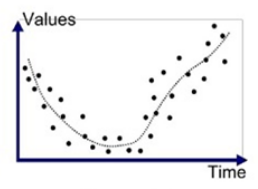
单神经元模型和线性模型的关系如下:

TensorFlow2实现单神经元模型也就是在线性模型基础上,加上激活函数,比如softmax、relu函数。常见的激活函数介绍如下:激活函数
代码如下:from testData import * 中的testData见上一篇文章。testData
import numpy as np
import tensorflow as tf
from testData import *
import time

class SNN(tf.keras.Model):
    def __init__(self):
        super().__init__()
        self.line = tf.keras.layers.Dense(units=10,activation=tf.nn.softmax)  #一个神经元的全连接网络,激活函数是非线性的
        self.flatten = tf.keras.layers.Reshape(target_shape=(28*28,))  #把二维的矩阵展平为1维

    def call(self,inputs):
        x = self.flatten(inputs)  #拉平成一个大的一维向量
        x = self.line(x)   #经过第一个全连接层
        output = x
        return output

#主控程序,调用数据并训练模型
#定义超参数
num_epochs = 5  #每个元素重复训练的次数
batch_size = 50
learning_rate = 0.001

print('now begin the train, time is ')
print(time.strftime('%Y-%m-%d %H:%M:%S',time.localtime()))
model = SNN()
data_loader = MNISTLoader()
optimier = tf.keras.optimizers.Adam(learning_rate=learning_rate)

num_batches = int(data_loader.num_train_data//batch_size*num_epochs)
for batch_index in range(num_batches):
    X,y = data_loader.get_batch(batch_size)
    with tf.GradientTape() as tape:
        y_pred = model(X)
        loss = tf.keras.losses.sparse_categorical_crossentropy(y_true=y,y_pred=y_pred)
        loss = tf.reduce_sum(loss)
        print("batch %d: loss %f"%(batch_index,loss.numpy()))
    grads = tape.gradient(loss,model.variables)
    optimier.apply_gradients(grads_and_vars=zip(grads,model.variables))

print('now end the train, time is ')
print(time.strftime('%Y-%m-%d %H:%M:%S', time.localtime()))
#模型的评估
sparse_categorical_accuracy = tf.keras.metrics.SparseCategoricalAccuracy()
num_batches_test = int(data_loader.num_test_data//batch_size)  #把测试数据拆分成多批次,每个批次50张图片
for batch_index in range(num_batches_test):
    start_index,end_index = batch_index*batch_size,(batch_index+1)*batch_size
    y_pred = model.predict(data_loader.test_data[start_index:end_index])
    sparse_categorical_accuracy.update_state(
        y_true = data_loader.test_label[start_index:end_index],
        y_pred=y_pred
    )
print('test accuracy: %f'%sparse_categorical_accuracy.result())
print('now end the test, time is ')
print(time.strftime('%Y-%m-%d %H:%M:%S',time.localtime()))
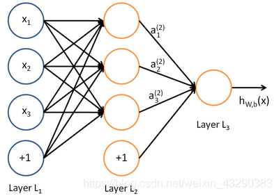
三、深度神经网络
深度神经网络可以理解成单神经网络的堆叠,中间可能会进行一些降维等处理,每一层的激活函数可以不同,因此有很多种组合,而且每层可以选择全连接、部分连接、随机连接等,非常多的组合。
结构如下:
代码如下(自己动手添加3层全连接层),from testData import * 中的testData见上一篇文章。testData
import numpy as np
import tensorflow as tf
from testData import *
import time

class DNN(tf.keras.Model):
    def __init__(self):
        super().__init__()
        self.dense1 = tf.keras.layers.Dense(units=50, activation=tf.nn.relu)  # 一个神经元的全连接网络,激活函数是非线性的
        self.dense2 = tf.keras.layers.Dense(units=100,activation=tf.nn.relu)  #一个神经元的全连接网络,激活函数是非线性的
        self.flatten = tf.keras.layers.Reshape(target_shape=(28*28,))  #把二维的矩阵展平为1维
        self.dense3 = tf.keras.layers.Dense(units=10, activation=tf.nn.softmax)  # 一个神经元的全连接网络,激活函数是非线性的

    def call(self,inputs):
        x = self.flatten(inputs)  #拉平成一个大的一维向量
        x = self.dense1(x)   #经过第一个全连接层
        x = self.dense2(x)  # 经过第2个全连接层
        x = self.dense3(x)  # 经过第3个全连接层
        output = x
        return output

#主控程序,调用数据并训练模型
#定义超参数
num_epochs = 5  #每个元素重复训练的次数
batch_size = 50
learning_rate = 0.001

print('now begin the train, time is ')
print(time.strftime('%Y-%m-%d %H:%M:%S',time.localtime()))
model = DNN()
data_loader = MNISTLoader()
optimier = tf.keras.optimizers.Adam(learning_rate=learning_rate)

num_batches = int(data_loader.num_train_data//batch_size*num_epochs)
for batch_index in range(num_batches):
    X,y = data_loader.get_batch(batch_size)
    with tf.GradientTape() as tape:
        y_pred = model(X)
        loss = tf.keras.losses.sparse_categorical_crossentropy(y_true=y,y_pred=y_pred)
        loss = tf.reduce_sum(loss)
        print("batch %d: loss %f"%(batch_index,loss.numpy()))
    grads = tape.gradient(loss,model.variables)
    optimier.apply_gradients(grads_and_vars=zip(grads,model.variables))

print('now end the train, time is ')
print(time.strftime('%Y-%m-%d %H:%M:%S', time.localtime()))
#模型的评估
sparse_categorical_accuracy = tf.keras.metrics.SparseCategoricalAccuracy()
num_batches_test = int(data_loader.num_test_data//batch_size)  #把测试数据拆分成多批次,每个批次50张图片
for batch_index in range(num_batches_test):
    start_index,end_index = batch_index*batch_size,(batch_index+1)*batch_size
    y_pred = model.predict(data_loader.test_data[start_index:end_index])
    sparse_categorical_accuracy.update_state(
        y_true = data_loader.test_label[start_index:end_index],
        y_pred=y_pred
    )
print('test accuracy: %f'%sparse_categorical_accuracy.result())
print('now end the test, time is ')
print(time.strftime('%Y-%m-%d %H:%M:%S',time.localtime()))
模型总结
通过线性模型和加上激活函数的单神经元模型对比可以看出,激活函数简直是神来之笔,一下子把准确率提升很多。
在图像识别领域,多神经网络的准确率比不上卷积神经网络,可能是因为过拟合导致的。