本文总结了mobilenet v1 v2 v3的网络结构特点,并通过tensorflow2.x以tf.keras的方式实现了mobilenet v2 v3。其中,mobilenet v3代码包含large和small两个模型,所以本文包含3个模型的代码实现,所有模型都包含通道缩放因子,可以搭建更小的模型,所有模型都包含完整的迁移学习代码,如果需要官方权重,可以自己通过tensorflow中的tf.keras.applications.mobilenetVX定义网络,然后通过model.save_weights()获得权重。mobilenet v1在本文中并未实现,但是可以参考【3】实现,mobilenet v2模型的实现参考了【4】【5】,mobilenet v3模型的实现参考了tensorflow官方代码【6】。其实tensorflow官方已经实现了v1 v2 v3的代码,可以直接调用,但是自己手动实现一遍可以加深对网络结构的理解,以及进行自定义网络结构修改。
mobilenet v1 v2 v3的网络结构特点

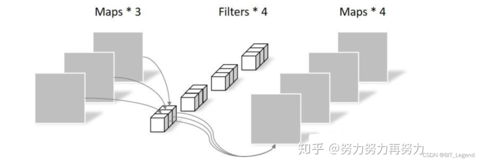
1. Mobilenet v1模型的核心是深度可分离卷积。
- 深度可分离卷积就是将原本标准的卷积操作因式分解成一个depthwise convolution和一个1*1的pointwise convolution操作,简单讲就是将原来一个卷积层分成两个卷积层,其中前面一个卷积层的每个filter都只跟input的每个channel进行卷积,然后后面一个卷积层则负责combining,即将上一层卷积的结果进行合并,与普通卷积相比深度可分离卷积能够将卷积层的计算量降低到1/8~1/9。v1版本中并未采用resnet的短接结构。

2. Mobilenet v2模型的核心是Inverted residuals(倒置残差)和Linear bottlenecks(线性瓶颈)。
- 倒置残差是指通常的residuals block是通过1*1的卷积核将通道减小,再经过3*3卷积,最后再通过1*1的卷积核从而将通道数扩大回去,从而减少计算量。而Inverted residuals刚好相反,通过先扩大通道数再进行卷积,最后再缩小回原来的通道数,基本思想就是,通过将通道数扩大,从而在中间层学到更多的特征,最后再总结筛选出优秀的特征出来。这么做的原因是:在 ResNet 中,使用的是标准的卷积层,如果不先用 1x1 conv 降低通道数,中间的 3x3 conv 计算量太大,因此,我们一般称这种 Residual Block 为 Bottleneck Block,即两头大中间小。但是在 MobileNet V2 中,中间的 3x3 conv 是深度级可分离卷积,计算量相比于标准卷积小很多,因此,为了提取更多特征,我们先用 1x1 conv 提升通道数,最后再用 1x1 conv 把通道数降下来,形成一种两头小中间大的模块,这与 Residual Block 是相反的。
- 为了避免Relu函数对特征的损失,在最后经过1*1的卷积缩小通道数后,放弃采用Relu激活函数,而是采用线性激活函数,在进行Eltwise sum操作,基本思想便是:在经历了1*1的卷积,降低通道数,这个已经使某些信息丢失,此外,当特征通道数变小,大部分的值都会趋向小于0,最后经过Relu激活函数,将再导致丢失一些特征信息。

![]()

MobileNet-V1 最大的特点就是采用depth-wise separable convolution来减少运算量以及参数量,而在网络结构上,没有采用shortcut的方式。
Resnet及Densenet等一系列采用shortcut的网络的成功,表明了shortcut是个非常好的东西,于是MobileNet-V2就将这个好东西拿来用。拿来主义,最重要的就是要结合自身的特点,MobileNet的特点就是depth-wise separable convolution,但是直接把depth-wise separable convolution应用到 residual block中,会碰到如下问题:
(1).DWConv layer层提取得到的特征受限于输入的通道数,若是采用以往的residual block,先“压缩”,再卷积提特征,那么DWConv layer可提取得特征就太少了,因此一开始不“压缩”,MobileNetV2反其道而行,一开始先“扩张”,本文实验“扩张”倍数为6。 通常residual block里面是 “压缩”→“卷积提特征”→“扩张”,MobileNetV2就变成了 “扩张”→“卷积提特征”→ “压缩”,因此称为Inverted residuals
(2).当采用“扩张”→“卷积提特征”→ “压缩”时,在“压缩”之后会碰到一个问题,那就是Relu会破坏特征。为什么这里的Relu会破坏特征呢?这得从Relu的性质说起,Relu对于负的输入,输出全为零;而本来特征就已经被“压缩”,再经过Relu的话,又要“损失”一部分特征,因此这里不采用Relu,实验结果表明这样做是正确的,这就称为Linear bottlenecks
3. Mobilenet v3模型的核心是轻量级的注意力模型、模型输入输出端缩减和h-swish代替swish函数。这个模型是基于AutoML构建,再人工微调对搜索结果进行优化,搜索方法使用了platform-aware NAS以及NetAdapt,分别用于全局搜索以及局部搜索,而人工微调则调整了网络前后几层的结构、bottleneck加入SE模块以及提出计算高效的h-swish非线性激活。
- MobileNetV2模型中反转残差结构和变量利用了1*1卷积来构建最后层,以便于拓展到高维的特征空间,虽然对于提取丰富特征进行预测十分重要,但却引入了二外的计算开销与延时。为了在保留高维特征的前提下减小延时,将平均池化前的层移除并用1x1卷积来计算特征图。特征生成层被移除后,先前用于瓶颈映射的层也不再需要了,这将为减少10ms的开销,在提速15%的同时减小了30m的操作数。
- 作者发现swish激活函数能够有效提高网络的精度。然而,swish的计算量太大了。作者提出h-swish(hard version of swish)这种非线性在保持精度的情况下带了了很多优势,首先ReLU6在众多软硬件框架中都可以实现,其次量化时避免了数值精度的损失,运行快。这一非线性改变将模型的延时增加了15%。但它带来的网络效应对于精度和延时具有正向促进,剩下的开销可以通过融合非线性与先前层来消除。

4. mobilenet v1 v2 v3效果对比。上图为SSDLite在使用mobilenet网络作为骨干网络时的检测精度和耗时情况,可以发现mobilenet v1 v2 v3large在检测精度上相差不大,但是在耗时上相差明显,v3small在检测精度上有一定的减小,但是耗时上优势相当明显。
MobileNet系列是很重要的轻量级网络家族,MobileNetV1使用深度可分离卷积来构建轻量级网络,MobileNetV2提出创新的inverted residual with linear bottleneck单元,虽然层数变多了,但是整体网络准确率和速度都有提升,MobileNetV3则结合AutoML技术以及人工微调进行更轻量级的网络构建。
mobilenet v2的代码实现(tf2.x或tf.keras)
# 通过tf.keras实现自定义的mobilenetv2网络
import tensorflow as tf
from tensorflow.keras import layers, models
from tensorflow.keras.layers import Conv2D, DepthwiseConv2D, Dense, Dropout, BatchNormalization, ReLU
from tensorflow.keras.layers import Input, GlobalAveragePooling2D, ZeroPadding2D
from tensorflow.keras.optimizers import Adam

############################################################################################################
## 0. 参数设置 ##############################################################################################
############################################################################################################

IMG_SIZE = (128, 128)
BATCH_SIZE = 128
CLASS_NUM = 7
alpha = 1.0           # 模型通道缩放系数

############################################################################################################
## 1. 搭建网络结构 ###########################################################################################
############################################################################################################

# 保证特征层数为8的倍数,输入为v和divisor,v是除数,divisor是被除数,将输出值改造为最接近v的divisor的倍数
def make_divisible(v, divisor, min_value=None):
    if min_value is None:
        min_value = divisor
    new_v = max(min_value, int(v+divisor/2)//divisor*divisor)   # 四舍五入取倍数值
    if new_v < 0.9*v:
        new_v += divisor
    return new_v

# 在stride等于2时,计算pad的上下左右尺寸,注:在stride等于1时,无需这么麻烦,直接就是correct,本函数仅仅针对stride=2
def pad_size(inputs, kernel_size):
    input_size = inputs.shape[1:3]
    if isinstance(kernel_size, int):
        kernel_size = (kernel_size, kernel_size)
    if input_size[0] is None:
        adjust = (1,1)
    else:
        adjust = (1- input_size[0]%2, 1-input_size[1]%2)
    correct = (kernel_size[0]//2, kernel_size[1]//2)
    return ((correct[0] - adjust[0], correct[0]),
            (correct[1] - adjust[1], correct[1]))

# 定义基本的卷积模块
def conv_block(x, nb_filter, kernel=(1,1), stride=(1,1), name=None):
    x = Conv2D(nb_filter, kernel, strides=stride, padding='same', use_bias=False, name=name+'_expand')(x)
    x = BatchNormalization(axis=3, name=name+'_expand_BN')(x, training=False)
    # x = Activation(relu6, name=name+'_expand_relu')(x)  # 采用这种Activation+自定义relu6的方式实现激活函数将导致后面无法量化感知训练
    x = ReLU(max_value=6.0, name=name+'_expand_relu')(x)
    return x

# 定义特有的残差卷积模块
def depthwise_res_block(x, nb_filter, kernel, stride, t, alpha, resdiual=False, name=None):
    # 准备工作
    input_tensor = x                        # 分一只出来等着残差结构的链接
    exp_channels = x.shape[-1]*t            # V2中特有的扩展维度,即先扩展维度再深度可分离卷积再缩小维度
    alpha_channels = int(nb_filter*alpha)   # 压缩维度,针对v2中几乎所有卷积层进行通道维度的压缩,从整个结构的第一层就开始了
    # 特有机构中的第一个卷积层,起到扩展维度的作用
    x = conv_block(x, exp_channels, (1,1), (1,1), name=name)
    # 在深度可分离卷积前,依据stride进行padding操作
    if stride[0] == 2:
        x = ZeroPadding2D(padding=pad_size(x, 3), name=name+'_pad')(x)
    # 进行深度可分离卷积操作,这里没有用集成函数,所以分两步进行卷积
    x = DepthwiseConv2D(kernel, padding='same' if stride[0]==1 else 'valid', strides=stride, depth_multiplier=1, use_bias=False, name=name+'_depthwise')(x)
    x = BatchNormalization(axis=3, name=name+'_depthwise_BN')(x, training=False)
    x = ReLU(max_value=6.0, name=name+'_depthwise_relu')(x)
    # 深度可分离中的第二步,可以减小维度
    x = Conv2D(alpha_channels, (1,1), padding='same', use_bias=False, strides=(1,1), name=name+'_project')(x)
    x = BatchNormalization(axis=3, name=name+'_project_BN')(x, training=False)
    # 是否需要残差结构,如果有残差,需要深度维度一致才能相加
    if resdiual:
        x = layers.add([x, input_tensor], name=name+'_add')
    return x

# 定义整个v2结构,特色就是独有的残差模块
def MovblieNetV2(img_size, nb_classes, alpha=1.0, dropout=0):
    # 输入端口
    img_input = Input(shape=img_size+(3,))
    # 第一个卷积模块是普通卷积
    first_filter = make_divisible(32*alpha, 8)
    x = ZeroPadding2D(padding=pad_size(img_input, 3), name='Conv1_pad')(img_input)
    x = Conv2D(first_filter, (3,3), strides=(2,2), padding='valid', use_bias=False, name='Conv1')(x)
    x = BatchNormalization(axis=3, name='bn_Conv1')(x, training=False)
    x = ReLU(max_value=6.0, name='Conv1_relu')(x)
    # 第一个深度可分离卷积模块,由于膨胀系数等于1,与剩余的深度可分离模块不兼容,所以无法使用depthwise_res_block函数
    x = DepthwiseConv2D((3,3), padding='same', strides=(1,1), depth_multiplier=1, use_bias=False, name='expanded_conv_depthwise')(x)
    x = BatchNormalization(axis=3, name='expanded_conv_depthwise_BN')(x, training=False)
    x = ReLU(max_value=6.0, name='expanded_conv_depthwise_relu')(x)
    x = Conv2D(16, (1,1), padding='same', use_bias=False, strides=(1,1), name='expanded_conv_project')(x)
    x = BatchNormalization(axis=3, name='expanded_conv_project_BN')(x, training=False)
    # 第二组特有深度可分离卷积组
    x = depthwise_res_block(x, 24, (3,3), (2,2), 6, alpha, resdiual=False, name='block_1')
    x = depthwise_res_block(x, 24, (3,3), (1,1), 6, alpha, resdiual=True, name='block_2')
    # 第三组特有深度可分离卷积组
    x = depthwise_res_block(x, 32, (3,3), (2,2), 6, alpha, resdiual=False, name='block_3')
    x = depthwise_res_block(x, 32, (3,3), (1,1), 6, alpha, resdiual=True, name='block_4')
    x = depthwise_res_block(x, 32, (3,3), (1,1), 6, alpha, resdiual=True, name='block_5')
    # 第四组特有深度可分离卷积组
    x = depthwise_res_block(x, 64, (3,3), (2,2), 6, alpha, resdiual=False, name='block_6')
    x = depthwise_res_block(x, 64, (3,3), (1,1), 6, alpha, resdiual=True, name='block_7')
    x = depthwise_res_block(x, 64, (3,3), (1,1), 6, alpha, resdiual=True, name='block_8')
    x = depthwise_res_block(x, 64, (3,3), (1,1), 6, alpha, resdiual=True, name='block_9')
    # 第五组特有深度可分离卷积组
    x = depthwise_res_block(x, 96, (3,3), (1,1), 6, alpha, resdiual=False, name='block_10')
    x = depthwise_res_block(x, 96, (3,3), (1,1), 6, alpha, resdiual=True, name='block_11')
    x = depthwise_res_block(x, 96, (3,3), (1,1), 6, alpha, resdiual=True, name='block_12')
    # 第六组特有深度可分离卷积组
    x = depthwise_res_block(x, 160, (3,3), (2,2), 6, alpha, resdiual=False, name='block_13')
    x = depthwise_res_block(x, 160, (3,3), (1,1), 6, alpha, resdiual=True, name='block_14')
    x = depthwise_res_block(x, 160, (3,3), (1,1), 6, alpha, resdiual=True, name='block_15')
    # 第七组特有深度可分离卷积组
    x = depthwise_res_block(x, 320, (3,3), (1,1), 6, alpha, resdiual=False, name='block_16')
    # 通道数计算
    if alpha > 1.0:
        last_filter = make_divisible(1280*alpha,8)
    else:
        last_filter = 1280
    # 特征提取网络的最后一个卷积是普通卷积
    x = Conv2D(last_filter, (1,1), strides=(1,1), use_bias=False, name='Conv_1')(x)
    x = BatchNormalization(axis=3, name='Conv_1_bn')(x, training=False)
    x = ReLU(max_value=6.0, name='out_relu')(x)
    # 通过全局均值池化对接特征提取网络和特征分类网络
    x = GlobalAveragePooling2D()(x)
    # 特征分类网络
    x = Dropout(dropout)(x)
    x = Dense(nb_classes, activation='softmax', use_bias=True, name='Logits')(x)
    # 搭建keras模型
    model = models.Model(img_input, x, name='MobileNetV2')
    # 返回结果模型
    return model
    # 需要说明的是在定义网络结构时如果没有指定Dropout和BN层的training属性,那tf会根据所调用函数自动设置,例如调用fit函数则为True,调用evaluate和
    # predict函数则为False,调用__call__函数时,默认是False,但是可以手动设置。但是如果在定义网络结构时给予了具体布尔值,则不管调用任何函数,都按照
    # 实际设置的属性使用

# 生成整个网络模型
model = MovblieNetV2(IMG_SIZE, CLASS_NUM, alpha, 0.2)
model.summary()完整的训练代码见:https://github.com/LegendBIT/tensorflow2.x-classification-model
mobilenet v2的代码实现(torch)
# 修改的mobilenetv2的网络模型 https://github.com/WZMIAOMIAO/deep-learning-for-image-processing
# 权重文件下载 download url: https://download.pytorch.org/models/mobilenet_v2-b0353104.pth
from torch import nn
import torch


# 设定整个模型的所有BN层的衰减系数,该系数用于平滑统计的均值和方差,torch与tf不太一样,两者以1为互补
momentum = 0.01  # 官方默认0.1,越小,最终的统计均值和方差越接近于整体均值和方差,前提是batchsize足够大

# 保证ch可以被8整除
def _make_divisible(ch, divisor=8, min_ch=None):
    if min_ch is None:
        min_ch = divisor
    new_ch = max(min_ch, int(ch + divisor / 2) // divisor * divisor)
    if new_ch < 0.9 * ch:
        new_ch += divisor
    return new_ch

# 定义基本卷积模块
class ConvBNReLU(nn.Sequential):
    def __init__(self, in_channel, out_channel, kernel_size=3, stride=1, groups=1):
        padding = (kernel_size - 1) // 2
        super(ConvBNReLU, self).__init__(
            nn.Conv2d(in_channel, out_channel, kernel_size, stride, padding, groups=groups, bias=False),
            nn.BatchNorm2d(out_channel, momentum=momentum),
            nn.ReLU6(inplace=True)
        )

# 定义mobilenetv2的基本模块
class InvertedResidual(nn.Module):
    def __init__(self, in_channel, out_channel, stride, expand_ratio):  # python并不要求子类一定要调用父类的构造函数
        super(InvertedResidual, self).__init__()     # 调用父类的构造函数,这里必须调用,父类的构造函数里有必须运行的代码
        hidden_channel = in_channel * expand_ratio
        self.use_shortcut = stride == 1 and in_channel == out_channel

        layers = []
        if expand_ratio != 1:
            # 1x1 pointwise conv
            layers.append(ConvBNReLU(in_channel, hidden_channel, kernel_size=1))
        layers.extend([
            # 3x3 depthwise conv
            ConvBNReLU(hidden_channel, hidden_channel, stride=stride, groups=hidden_channel),
            # 1x1 pointwise conv(linear)
            nn.Conv2d(hidden_channel, out_channel, kernel_size=1, bias=False),
            nn.BatchNorm2d(out_channel, momentum=momentum),
        ])

        self.conv = nn.Sequential(*layers)

    def forward(self, x):
        if self.use_shortcut:
            return x + self.conv(x)
        else:
            return self.conv(x)

# 定义模型
class MobileNetV2(nn.Module):
    def __init__(self, num_classes=1000, alpha=1.0, round_nearest=8):
        super(MobileNetV2, self).__init__()
        block = InvertedResidual
        input_channel = _make_divisible(32 * alpha, round_nearest)
        last_channel = _make_divisible(1280 * alpha, round_nearest)

        inverted_residual_setting = [
            # t, c, n, s
            [1, 16, 1, 1],
            [6, 24, 2, 2],
            [6, 32, 3, 2],
            [6, 64, 4, 2],
            [6, 96, 3, 1],
            [6, 160, 3, 2],
            [6, 320, 1, 1],
        ]

        features = []
        # 定义第一层网络
        features.append(ConvBNReLU(3, input_channel, stride=2))
        # 定义所有残差模块
        for t, c, n, s in inverted_residual_setting:
            output_channel = _make_divisible(c * alpha, round_nearest)
            for i in range(n):
                stride = s if i == 0 else 1
                features.append(block(input_channel, output_channel, stride, expand_ratio=t))
                input_channel = output_channel
        # 定义backbone的最后一层
        features.append(ConvBNReLU(input_channel, last_channel, 1))
        # 定义完整的backbone模型
        self.features = nn.Sequential(*features)

        # 定义最后的分类层
        self.avgpool = nn.AdaptiveAvgPool2d((1, 1))
        self.classifier = nn.Sequential(
            nn.Dropout(0.2),
            nn.Linear(last_channel, num_classes)
        )

        # 模型权重初始化
        for m in self.modules():
            if isinstance(m, nn.Conv2d):
                nn.init.kaiming_normal_(m.weight, mode='fan_out')
                if m.bias is not None:
                    nn.init.zeros_(m.bias)
            elif isinstance(m, nn.BatchNorm2d):
                nn.init.ones_(m.weight)
                nn.init.zeros_(m.bias)
            elif isinstance(m, nn.Linear):
                nn.init.normal_(m.weight, 0, 0.01)
                nn.init.zeros_(m.bias)

    def forward(self, x):
        x = self.features(x)
        x = self.avgpool(x)
        x = torch.flatten(x, 1)  # 类比view()是改变维度,torch.flatten(input, start_dim=0, end_dim=-1) 是拉伸维度
        x = self.classifier(x)   # torch.transpose(input, dim0, dim1)是交换维度
return x # 最后的输出层并不包含激活函数,直接就是全链接的输出,在损失函数中包含softmax操作,实际使用需要自己再加一个softmax完整的训练代码见:https://github.com/LegendBIT/torch-classification-model
mobilenet v3的代码实现(tf2.x或tf.keras)
# 根据tf.keras的官方代码修改的mobilenetv3的网络模型
import tensorflow as tf
from tensorflow.keras import layers, models


"""
    Reference:
    - [Searching for MobileNetV3](https://arxiv.org/pdf/1905.02244.pdf) (ICCV 2019)
    The following table describes the performance of MobileNets v3:
    ------------------------------------------------------------------------
    MACs stands for Multiply Adds
    |Classification Checkpoint|MACs(M)|Parameters(M)|Top1 Accuracy|Pixel1 CPU(ms)|
    |---|---|---|---|---|
    | mobilenet_v3_large_1.0_224              | 217 | 5.4 |   75.6   |   51.2  |
    | mobilenet_v3_large_0.75_224             | 155 | 4.0 |   73.3   |   39.8  |
    | mobilenet_v3_large_minimalistic_1.0_224 | 209 | 3.9 |   72.3   |   44.1  |
    | mobilenet_v3_small_1.0_224              | 66  | 2.9 |   68.1   |   15.8  |
    | mobilenet_v3_small_0.75_224             | 44  | 2.4 |   65.4   |   12.8  |
    | mobilenet_v3_small_minimalistic_1.0_224 | 65  | 2.0 |   61.9   |   12.2  |
    For image classification use cases, see
    [this page for detailed examples](https://keras.io/api/applications/#usage-examples-for-image-classification-models).
    For transfer learning use cases, make sure to read the
    [guide to transfer learning & fine-tuning](https://keras.io/guides/transfer_learning/).
"""

##################################################################################################################################
# 定义V3的完整模型 #################################################################################################################
##################################################################################################################################
def MobileNetV3(input_shape=[224, 224 ,3], classes=1000, dropout_rate=0.2, alpha=1.0, weights=None,
                 model_type='large', minimalistic=False, classifier_activation='softmax', include_preprocessing=False):
    # 如果有权重文件,那就意味着要迁移学习,那就意味着需要让BN层始终处于infer状态,否则解冻整个网络后,会出现acc下降loss上升的现象,终其原因是解冻网络之
    # 前,网络BN层用的是之前数据集的均值和方差,解冻后虽然维护着新的滑动平均和滑动方差,但是单次训练时使用的是当前batch的均值和方差,差异太大造成特征崩塌
    if weights:
        bn_training = False
    else:
        bn_training = None
    bn_decay = 0.99  # BN层的滑动平均系数,这个值的设置需要匹配steps和batchsize否则会出现奇怪现象
    # 确定通道所处维度
    channel_axis = -1
    # 根据是否为mini设置,修改部分配置参数
    if minimalistic:
        kernel = 3
        activation = relu
        se_ratio = None
        name = "mini"
    else:
        kernel = 5
        activation = hard_swish
        se_ratio = 0.25
        name = "norm"
    # 定义模型输入张量
    img_input = layers.Input(shape=input_shape)
    # 是否包含预处理层
    if include_preprocessing:
        x = layers.Rescaling(scale=1. / 127.5, offset=-1.)(img_input)
    else:
        x = img_input
    # 定义整个模型的第一个特征提取层
    x = layers.Conv2D(16, kernel_size=3, strides=(2, 2), padding='same', use_bias=False, name='Conv')(x)
    x = layers.BatchNormalization(axis=channel_axis, epsilon=1e-3, momentum=bn_decay, name='Conv/BatchNorm')(x, training=bn_training)
    x = activation(x)
    # 定义整个模型的骨干特征提取
    if model_type == 'large':
        x = MobileNetV3Large(x, kernel, activation, se_ratio, alpha, bn_training, bn_decay)
        last_point_ch = 1280
    else:
        x = MobileNetV3Small(x, kernel, activation, se_ratio, alpha, bn_training, bn_decay)
        last_point_ch = 1024
    # 定义整个模型的后特征提取
    last_conv_ch = _depth(x.shape[channel_axis] * 6)
    # if the width multiplier is greater than 1 we increase the number of output channels
    if alpha > 1.0:
        last_point_ch = _depth(last_point_ch * alpha)
    x = layers.Conv2D(last_conv_ch, kernel_size=1, padding='same', use_bias=False, name='Conv_1')(x)
    x = layers.BatchNormalization(axis=channel_axis, epsilon=1e-3, momentum=bn_decay, name='Conv_1/BatchNorm')(x, training=bn_training)
    x = activation(x)
    # 如果tf版本大于等于2.6则直接使用下面第一句就可以了,否则使用下面2~3句
    # x = layers.GlobalAveragePooling2D(data_format='channels_last', keepdims=True)(x)
    x = layers.GlobalAveragePooling2D(data_format='channels_last')(x)
    x= tf.expand_dims(tf.expand_dims(x, 1), 1)
    # 定义第一个特征分类层
    x = layers.Conv2D(last_point_ch, kernel_size=1, padding='same', use_bias=True, name='Conv_2')(x)
    x = activation(x)
    # 定义第二个特征分类层
    if dropout_rate > 0:
        x = layers.Dropout(dropout_rate)(x)
    x = layers.Conv2D(classes, kernel_size=1, padding='same', name='Logits')(x)
    x = layers.Flatten()(x)
    x = layers.Activation(activation=classifier_activation, name='Predictions')(x)  # 注意损失函数需要与初始权重匹配,否则预训练没有意义
    # 创建模型
    model = models.Model(img_input, x, name='MobilenetV3' + '_' + model_type + '_' + name)
    # 恢复权重
    if weights:
        model.load_weights(weights, by_name=True)
        # print(model.get_layer(name="block_8_project_BN").get_weights()[0][:4])

    return model


##################################################################################################################################
# 定义V3的骨干网络,不包含前处理和后处理 ###############################################################################################
##################################################################################################################################

# 定义mobilenetv3-small的骨干部分,不包含第一层的卷积特征提取和后处理
def MobileNetV3Small(x, kernel, activation, se_ratio, alpha, bn_training, mome):

    def depth(d):
      return _depth(d * alpha)

    x = _inverted_res_block(x, 1, depth(16), 3, 2, se_ratio, relu, 0, bn_training, mome)
    x = _inverted_res_block(x, 72. / 16, depth(24), 3, 2, None, relu, 1, bn_training, mome)
    x = _inverted_res_block(x, 88. / 24, depth(24), 3, 1, None, relu, 2, bn_training, mome)
    x = _inverted_res_block(x, 4, depth(40), kernel, 2, se_ratio, activation, 3, bn_training, mome)
    x = _inverted_res_block(x, 6, depth(40), kernel, 1, se_ratio, activation, 4, bn_training, mome)
    x = _inverted_res_block(x, 6, depth(40), kernel, 1, se_ratio, activation, 5, bn_training, mome)
    x = _inverted_res_block(x, 3, depth(48), kernel, 1, se_ratio, activation, 6, bn_training, mome)
    x = _inverted_res_block(x, 3, depth(48), kernel, 1, se_ratio, activation, 7, bn_training, mome)
    x = _inverted_res_block(x, 6, depth(96), kernel, 2, se_ratio, activation, 8, bn_training, mome)
    x = _inverted_res_block(x, 6, depth(96), kernel, 1, se_ratio, activation, 9, bn_training, mome)
    x = _inverted_res_block(x, 6, depth(96), kernel, 1, se_ratio, activation, 10, bn_training, mome)

    return x

# 定义mobilenetv3-large的骨干部分,不包含第一层的卷积特征提取和后处理
def MobileNetV3Large(x, kernel, activation, se_ratio, alpha, bn_training, mome):

    def depth(d):
        return _depth(d * alpha)

    x = _inverted_res_block(x, 1, depth(16), 3, 1, None, relu, 0, bn_training, mome)
    x = _inverted_res_block(x, 4, depth(24), 3, 2, None, relu, 1, bn_training, mome)
    x = _inverted_res_block(x, 3, depth(24), 3, 1, None, relu, 2, bn_training, mome)
    x = _inverted_res_block(x, 3, depth(40), kernel, 2, se_ratio, relu, 3, bn_training, mome)
    x = _inverted_res_block(x, 3, depth(40), kernel, 1, se_ratio, relu, 4, bn_training, mome)
    x = _inverted_res_block(x, 3, depth(40), kernel, 1, se_ratio, relu, 5, bn_training, mome)
    x = _inverted_res_block(x, 6, depth(80), 3, 2, None, activation, 6, bn_training, mome)
    x = _inverted_res_block(x, 2.5, depth(80), 3, 1, None, activation, 7, bn_training, mome)
    x = _inverted_res_block(x, 2.3, depth(80), 3, 1, None, activation, 8, bn_training, mome)
    x = _inverted_res_block(x, 2.3, depth(80), 3, 1, None, activation, 9, bn_training, mome)
    x = _inverted_res_block(x, 6, depth(112), 3, 1, se_ratio, activation, 10, bn_training, mome)
    x = _inverted_res_block(x, 6, depth(112), 3, 1, se_ratio, activation, 11, bn_training, mome)
    x = _inverted_res_block(x, 6, depth(160), kernel, 2, se_ratio, activation, 12, bn_training, mome)
    x = _inverted_res_block(x, 6, depth(160), kernel, 1, se_ratio, activation, 13, bn_training, mome)
    x = _inverted_res_block(x, 6, depth(160), kernel, 1, se_ratio, activation, 14, bn_training, mome)

    return x


##################################################################################################################################
# 定义V3的骨干模块 #################################################################################################################
##################################################################################################################################

# 定义relu函数
def relu(x):
    return layers.ReLU()(x)

# 定义sigmoid函数的近似函数h-sigmoid函数
def hard_sigmoid(x):
    return layers.ReLU(6.)(x + 3.) * (1. / 6.)

# 定义swish函数的近似函数,替换原本的sigmoid函数为新的h-sigmoid函数
def hard_swish(x):
    return layers.Multiply()([x, hard_sigmoid(x)])

# python中变量前加单下划线:是提示程序员该变量或函数供内部使用,但不是强制的,只是提示,但是不能用“from xxx import *”而导入
# python中变量后加单下划线:是避免变量名冲突
# python中变量前加双下划线:是强制该变量或函数供类内部使用,名称会被强制修改,所以原名称无法访问到,新名称可以访问到,所以也不是外部完全无法访问
# python中变量前后双下划线:是用于类内部定义使用,是特殊用途,外部可以直接访问,平时程序员不要这样定义
# 通过函数实现不管v为多大,输出new_v始终能够被divisor整除,且new_v是大于等于min_value且不能太小的四舍五入最接近divisor整除的数
def _depth(v, divisor=8, min_value=None):
    if min_value is None:
        min_value = divisor
    # 保证new_v一定大于等于min_value,max中第二个值保证是v的四舍五入的能够被divisor整除的数
    new_v = max(min_value, int(v + divisor / 2) // divisor * divisor)
    # 保证new_v不要太小
    if new_v < 0.9 * v:
        new_v += divisor
    return new_v

# 在stride等于2时,计算pad的上下左右尺寸,注:在stride等于1时,无需这么麻烦,直接就是correct,本函数仅仅针对stride=2
def pad_size(inputs, kernel_size):
    input_size = inputs.shape[1:3]
    if isinstance(kernel_size, int):
        kernel_size = (kernel_size, kernel_size)
    if input_size[0] is None:
        adjust = (1,1)
    else:
        adjust = (1- input_size[0]%2, 1-input_size[1]%2)
    correct = (kernel_size[0]//2, kernel_size[1]//2)
    return ((correct[0] - adjust[0], correct[0]),
            (correct[1] - adjust[1], correct[1]))

# 定义通道注意力机制模块,这里filters数字应该是要等于inputs的通道数的,否则最后一步的相乘无法完成,se_ratio可以调节缩放比例
def _se_block(inputs, filters, se_ratio, prefix):
    # 如果tf版本大于等于2.6则直接使用下面第一句就可以了,否则使用下面2~3句
    # x = layers.GlobalAveragePooling2D(data_format='channels_last', keepdims=True, name=prefix + 'squeeze_excite/AvgPool')(inputs)
    x = layers.GlobalAveragePooling2D(data_format='channels_last', name=prefix + 'squeeze_excite/AvgPool')(inputs)
    x= tf.expand_dims(tf.expand_dims(x, 1), 1)
    x = layers.Conv2D(_depth(filters * se_ratio), kernel_size=1, padding='same', name=prefix + 'squeeze_excite/Conv')(x)
    x = layers.ReLU(name=prefix + 'squeeze_excite/Relu')(x)
    x = layers.Conv2D(filters, kernel_size=1, padding='same', name=prefix + 'squeeze_excite/Conv_1')(x)
    x = hard_sigmoid(x)
    x = layers.Multiply(name=prefix + 'squeeze_excite/Mul')([inputs, x])
    return x

# 定义V3的基础模块,可以通过expansion调整模块中所有特整层的通道数,se_ratio可以调节通道注意力机制中的缩放系数
def _inverted_res_block(x, expansion, filters, kernel_size, stride, se_ratio, activation, block_id, bn_training, mome):
    channel_axis = -1  # 在tf中通道维度是最后一维
    shortcut = x
    prefix = 'expanded_conv/'
    infilters = x.shape[channel_axis]
    if block_id:
        prefix = 'expanded_conv_{}/'.format(block_id)
        x = layers.Conv2D(_depth(infilters * expansion), kernel_size=1, padding='same', use_bias=False, name=prefix + 'expand')(x)
        x = layers.BatchNormalization(axis=channel_axis, epsilon=1e-3, momentum=mome, name=prefix + 'expand/BatchNorm')(x, training=bn_training)
        x = activation(x)

    if stride == 2:
        x = layers.ZeroPadding2D(padding=pad_size(x, kernel_size), name=prefix + 'depthwise/pad')(x)
    x = layers.DepthwiseConv2D(kernel_size, strides=stride, padding='same' if stride == 1 else 'valid', use_bias=False, name=prefix + 'depthwise')(x)
    x = layers.BatchNormalization(axis=channel_axis, epsilon=1e-3, momentum=mome, name=prefix + 'depthwise/BatchNorm')(x, training=bn_training)
    x = activation(x)

    if se_ratio:
        x = _se_block(x, _depth(infilters * expansion), se_ratio, prefix)

    x = layers.Conv2D(filters, kernel_size=1, padding='same', use_bias=False, name=prefix + 'project')(x)
    x = layers.BatchNormalization(axis=channel_axis, epsilon=1e-3, momentum=mome, name=prefix + 'project/BatchNorm')(x, training=bn_training)

    if stride == 1 and infilters == filters:
        x = layers.Add(name=prefix + 'Add')([shortcut, x])
    return x

## no.1
# 在keras中每个model以及model中的layer都存在trainable属性,如果将trainable属性设置为False,那么相应的model或者layer所对应
# 的参数将不会再改变,但是当前不建议直接对model操作,建议直接对layer进行操作,原因是当前有bug,对model设置后,有可能再对layer进
# 行操作就失效了。后面证明这个并非bug,而是model和layer都存在trainable属性,对model的设置会影响到layer的设置,但是对layer的
# 设置不会影响到model的设置,当首先设置model的trainable属性为False时,后面不管对layer的trainable属性怎么设置,都不会改变model
# 的trainable属性为False这一事实,当调用训练函数时,框架首先检查model的trainable属性,如果该属性为False,那就是终止训练,所以
# 不管内部的layer的trainable属性怎么设置都没用。此外,BN层和Dropout层还存在training的形参,这个形参是用来告诉对应层属于train
# 状态还是infer状态,例如BN层,其在train状态采用的是当前batch的均值和方差,并维护一个滑动平均的均值和方差,在infer状态采用的是之
# 前维护的滑动平均的均值和方差。原本trainable属性和training形参是相互独立的,但是在BN层这里是个例外,就是当BN层的最终trainable
# 属性为True时,一切正常,BN层的线性变换系数可以训练可以被修改,BN层的training设置也符合上面所述。但是当BN层的trainable属性为
# False时,就会出现问题,此时线性变换系数不可以训练不可以被修改,这个正常,但是此时BN层将处在infer状态,即trianing参数被修改为
# False,此时滑动均值和方差不会再修改,也就是说在调用fit()时,BN层将采用之前的滑动均值和方差进行计算,并不是当前batch的均值和方差,
# 且不会维护着滑动平均的均值和方差。这个造成的问题是在迁移学习时,从只是训练最后一层变换到训练整个网络时,整个误差和acc都会剧降,原因
# 就是在冻结训练时,BN层处在不可训练状态,那么其BN一直采用的是旧数据的均值和方差,且没有维护滑动平均的均值和方差,当变换到全网络训练时,
# BN层处在可训练状态,此时BN层采用的当前batch的的均值和方差,且开始维护着滑动平均的均值和方差,这会造成后面的分类层无法使用BN层中的
# 参数巨变,进而对识别精度产生重大影响。所以,问题的根本原因是在BN层处于不可训练状态时,其会自动处在infer状态,解决这一问题最简单的方式
# 是,在定义网络时直接把BN层的training设置为False,这样不管BN层处在何种状态,BN层都是采用旧数据的均值和方差进行计算,不会再更新,
# 这样就不会出现参数巨变也不会出现准确率剧降,也可以直接先计算一下新数据整体的均值和方差,然后在迁移学习时,先把方差和均值恢复进网络里,
# 同时training设置为False。关于BN与training参数和trainable属性的相互影响,详细见自己的CSDN博客。

## no.2
# 测试中间模型准确率,第一次调试时遇到一个问题就是当没有采用迁移学习而是整个网络随机初始化且同时训练时,fit在训练集上进行训练,acc
# 逐步提升很正常,但是同步在验证集和测试集上acc在前7~8轮训练完全不增加,最后增加了,也增加的相当有限,最后排查原因发现,是因为网络
# 中有BN结构造成的,BN结构中存在一个均值和方差,它们是通过步进平滑计算得到的,最终这两个值趋近于全部数据集的整体均值和方差
# (batchsize==1,平滑系数==0.99时,趋近于时间上最近的几百多个数据的类似平均,如果加大batchsize和增大平滑系数,最终趋近于整体的
# 均值和方差,所以其实也可以直接计算整体均值和方差然后赋值),但是如果刚开始训练时batchsize设置过大,而总数量不足将会导致训练完一轮
# 以后,steps数过小,如果此时平滑系数还很大,那步进计算的均值和方差将非常接近于初始的随机值而不是数据集的平均值,那在测试状态下,网
# 络的输出结果就很差,而在训练状态下,这个均值和方差是通过一个batch实时计算的,后面匹配的线性变换也是实时改变的,所以质量比较好,所
# 以才会出现同样是训练集fit时acc很好,但是evaluate时acc巨差的现象,所以在数据集比较小时,且不是迁移学习时,batchsize可以设置的
# 小一点以及滑动系数设置的小一点。

## no.3
# 需要说明的是在定义网络结构时如果没有指定Dropout和BN层的training属性,那tf会根据所调用函数自动设置,例如调用fit函数则为True,调用evaluate和
# predict函数则为False,调用__call__函数时,默认是False,但是可以手动设置。但是如果在定义网络结构时给予了具体布尔值,则不管调用任何函数,都按照
# 实际设置的属性使用

## no.4
# 更详细的讲解详见CSDN博客<BN(Batch Normalization) 的理论理解以及在tf.keras中的实际应用和总结>完整的训练代码见:https://github.com/LegendBIT/tensorflow2.x-classification-model
mobilenet v3的代码实现(torch)
# 修改的mobilenetv3的网络模型 https://github.com/WZMIAOMIAO/deep-learning-for-image-processing
# 权重文件下载 download url: https://download.pytorch.org/models/mobilenet_v3_large-8738ca79.pth
# 权重文件下载 download url: https://download.pytorch.org/models/mobilenet_v3_small-047dcff4.pth
from typing import Callable, List, Optional

import torch
from torch import nn, Tensor
from torch.nn import functional as F
from functools import partial

# 设定整个模型的所有BN层的衰减系数,该系数用于平滑统计的均值和方差,torch与tf不太一样,两者以1为互补
momentum = 0.01  # 官方默认0.1,越小,最终的统计均值和方差越接近于整体均值和方差,前提是batchsize足够大

# 保证ch可以被8整除
def _make_divisible(ch, divisor=8, min_ch=None):
    if min_ch is None:
        min_ch = divisor
    new_ch = max(min_ch, int(ch + divisor / 2) // divisor * divisor)
    if new_ch < 0.9 * ch:
        new_ch += divisor
    return new_ch

# 定义最小卷积模块,这个写法比较少见,一般都是继承nn.Module,然后在forward()函数中定义模型,或者直接利用nn.Sequential()定义模型
class ConvBNActivation(nn.Sequential):                       # 这种写法是直接利用nn.Sequential()定义模型的一种变种写法
    def __init__(self,
                 in_planes: int,
                 out_planes: int,
                 kernel_size: int = 3,
                 stride: int = 1,
                 groups: int = 1,
                 norm_layer: Optional[Callable[..., nn.Module]] = None,
                 activation_layer: Optional[Callable[..., nn.Module]] = None):
        padding = (kernel_size - 1) // 2
        if norm_layer is None:
            norm_layer = nn.BatchNorm2d
        if activation_layer is None:
            activation_layer = nn.ReLU6
        super(ConvBNActivation, self).__init__(nn.Conv2d(in_channels=in_planes,
                                                         out_channels=out_planes,
                                                         kernel_size=kernel_size,
                                                         stride=stride,
                                                         padding=padding,
                                                         groups=groups,
                                                         bias=False),
                                               norm_layer(out_planes),
                                               activation_layer(inplace=True))

# 定义SE模块,负责通道注意力机制
class SqueezeExcitation(nn.Module):
    def __init__(self, input_c: int, squeeze_factor: int = 4):
        super(SqueezeExcitation, self).__init__()
        squeeze_c = _make_divisible(input_c // squeeze_factor, 8)
        self.fc1 = nn.Conv2d(input_c, squeeze_c, 1)
        self.fc2 = nn.Conv2d(squeeze_c, input_c, 1)

    def forward(self, x: Tensor) -> Tensor:
        scale = F.adaptive_avg_pool2d(x, output_size=(1, 1))
        scale = self.fc1(scale)
        scale = F.relu(scale, inplace=True)
        scale = self.fc2(scale)
        scale = F.hardsigmoid(scale, inplace=True)
        return scale * x

# 定义一个配置类,只是用来存储配置参数
class InvertedResidualConfig:
    def __init__(self,
                 input_c: int,
                 kernel: int,
                 expanded_c: int,
                 out_c: int,
                 use_se: bool,
                 activation: str,
                 stride: int,
                 width_multi: float):
        self.input_c = self.adjust_channels(input_c, width_multi)
        self.kernel = kernel
        self.expanded_c = self.adjust_channels(expanded_c, width_multi)
        self.out_c = self.adjust_channels(out_c, width_multi)
        self.use_se = use_se
        self.use_hs = activation == "HS"  # whether using h-swish activation
        self.stride = stride

    @staticmethod
    def adjust_channels(channels: int, width_multi: float):
        return _make_divisible(channels * width_multi, 8)

# 定义基本模块-反残差结构
class InvertedResidual(nn.Module):
    def __init__(self, cnf: InvertedResidualConfig, norm_layer: Callable[..., nn.Module]):
        super(InvertedResidual, self).__init__()

        if cnf.stride not in [1, 2]:
            raise ValueError("illegal stride value.")

        self.use_res_connect = (cnf.stride == 1 and cnf.input_c == cnf.out_c)

        layers: List[nn.Module] = []
        activation_layer = nn.Hardswish if cnf.use_hs else nn.ReLU

        # expand
        if cnf.expanded_c != cnf.input_c:
            layers.append(ConvBNActivation(cnf.input_c,
                                           cnf.expanded_c,
                                           kernel_size=1,
                                           norm_layer=norm_layer,
                                           activation_layer=activation_layer))

        # depthwise
        layers.append(ConvBNActivation(cnf.expanded_c,
                                       cnf.expanded_c,
                                       kernel_size=cnf.kernel,
                                       stride=cnf.stride,
                                       groups=cnf.expanded_c,
                                       norm_layer=norm_layer,
                                       activation_layer=activation_layer))

        if cnf.use_se:
            layers.append(SqueezeExcitation(cnf.expanded_c))

        # project
        layers.append(ConvBNActivation(cnf.expanded_c,
                                       cnf.out_c,
                                       kernel_size=1,
                                       norm_layer=norm_layer,
                                       activation_layer=nn.Identity))

        self.block = nn.Sequential(*layers)
        self.out_channels = cnf.out_c
        self.is_strided = cnf.stride > 1

    def forward(self, x: Tensor) -> Tensor:
        result = self.block(x)
        if self.use_res_connect:
            result += x

        return result

# 定义公共模型模板
class MobileNetV3(nn.Module):
    def __init__(self,
                 inverted_residual_setting: List[InvertedResidualConfig],
                 last_channel: int,
                 num_classes: int = 1000,
                 block: Optional[Callable[..., nn.Module]] = None,
                 norm_layer: Optional[Callable[..., nn.Module]] = None):
        super(MobileNetV3, self).__init__()

        if not inverted_residual_setting:
            raise ValueError("The inverted_residual_setting should not be empty.")
        elif not (isinstance(inverted_residual_setting, List) and
                  all([isinstance(s, InvertedResidualConfig) for s in inverted_residual_setting])):
            raise TypeError("The inverted_residual_setting should be List[InvertedResidualConfig]")

        if block is None:
            block = InvertedResidual

        if norm_layer is None:
            norm_layer = partial(nn.BatchNorm2d, eps=0.001, momentum=momentum)

        layers: List[nn.Module] = []

        # building first layer
        firstconv_output_c = inverted_residual_setting[0].input_c
        layers.append(ConvBNActivation(3,
                                       firstconv_output_c,
                                       kernel_size=3,
                                       stride=2,
                                       norm_layer=norm_layer,
                                       activation_layer=nn.Hardswish))
        # building inverted residual blocks
        for cnf in inverted_residual_setting:
            layers.append(block(cnf, norm_layer))

        # building last several layers
        lastconv_input_c = inverted_residual_setting[-1].out_c
        lastconv_output_c = 6 * lastconv_input_c
        layers.append(ConvBNActivation(lastconv_input_c,
                                       lastconv_output_c,
                                       kernel_size=1,
                                       norm_layer=norm_layer,
                                       activation_layer=nn.Hardswish))
        self.features = nn.Sequential(*layers)
        self.avgpool = nn.AdaptiveAvgPool2d(1)
        self.classifier = nn.Sequential(nn.Linear(lastconv_output_c, last_channel),
                                        nn.Hardswish(inplace=True),
                                        nn.Dropout(p=0.2, inplace=True),
                                        nn.Linear(last_channel, num_classes))

        # initial weights
        for m in self.modules():
            if isinstance(m, nn.Conv2d):
                nn.init.kaiming_normal_(m.weight, mode="fan_out")
                if m.bias is not None:
                    nn.init.zeros_(m.bias)
            elif isinstance(m, (nn.BatchNorm2d, nn.GroupNorm)):
                nn.init.ones_(m.weight)
                nn.init.zeros_(m.bias)
            elif isinstance(m, nn.Linear):
                nn.init.normal_(m.weight, 0, 0.01)
                nn.init.zeros_(m.bias)

    def _forward_impl(self, x: Tensor) -> Tensor:
        x = self.features(x)
        x = self.avgpool(x)
        x = torch.flatten(x, 1)
        x = self.classifier(x)    # 最后的输出层并不包含激活函数,直接就是全链接的输出,在损失函数中包含softmax操作,实际使用需要自己再加一个softmax

        return x

    def forward(self, x: Tensor) -> Tensor:
        return self._forward_impl(x)

# 定义large结构
def mobilenet_v3_large(num_classes: int = 1000, width_multi: float = 1.0, reduced_tail: bool = False) -> MobileNetV3:
    """
    Constructs a large MobileNetV3 architecture from "Searching for MobileNetV3" <https://arxiv.org/abs/1905.02244>.
    """
    bneck_conf = partial(InvertedResidualConfig, width_multi=width_multi)
    adjust_channels = partial(InvertedResidualConfig.adjust_channels, width_multi=width_multi)

    reduce_divider = 2 if reduced_tail else 1

    inverted_residual_setting = [
        # input_c, kernel, expanded_c, out_c, use_se, activation, stride
        bneck_conf(16, 3, 16, 16, False, "RE", 1),
        bneck_conf(16, 3, 64, 24, False, "RE", 2),  # C1
        bneck_conf(24, 3, 72, 24, False, "RE", 1),
        bneck_conf(24, 5, 72, 40, True, "RE", 2),  # C2
        bneck_conf(40, 5, 120, 40, True, "RE", 1),
        bneck_conf(40, 5, 120, 40, True, "RE", 1),
        bneck_conf(40, 3, 240, 80, False, "HS", 2),  # C3
        bneck_conf(80, 3, 200, 80, False, "HS", 1),
        bneck_conf(80, 3, 184, 80, False, "HS", 1),
        bneck_conf(80, 3, 184, 80, False, "HS", 1),
        bneck_conf(80, 3, 480, 112, True, "HS", 1),
        bneck_conf(112, 3, 672, 112, True, "HS", 1),
        bneck_conf(112, 5, 672, 160 // reduce_divider, True, "HS", 2),  # C4
        bneck_conf(160 // reduce_divider, 5, 960 // reduce_divider, 160 // reduce_divider, True, "HS", 1),
        bneck_conf(160 // reduce_divider, 5, 960 // reduce_divider, 160 // reduce_divider, True, "HS", 1),
    ]
    last_channel = adjust_channels(1280 // reduce_divider)  # C5

    return MobileNetV3(inverted_residual_setting=inverted_residual_setting, last_channel=last_channel, num_classes=num_classes)

# 定义small结构
def mobilenet_v3_small(num_classes: int = 1000, width_multi: float = 1.0, reduced_tail: bool = False) -> MobileNetV3:
    """
    Constructs a large MobileNetV3 architecture from "Searching for MobileNetV3" <https://arxiv.org/abs/1905.02244>.
    """
    bneck_conf = partial(InvertedResidualConfig, width_multi=width_multi)
    adjust_channels = partial(InvertedResidualConfig.adjust_channels, width_multi=width_multi)

    reduce_divider = 2 if reduced_tail else 1

    inverted_residual_setting = [
        # input_c, kernel, expanded_c, out_c, use_se, activation, stride
        bneck_conf(16, 3, 16, 16, True, "RE", 2),  # C1
        bneck_conf(16, 3, 72, 24, False, "RE", 2),  # C2
        bneck_conf(24, 3, 88, 24, False, "RE", 1),
        bneck_conf(24, 5, 96, 40, True, "HS", 2),  # C3
        bneck_conf(40, 5, 240, 40, True, "HS", 1),
        bneck_conf(40, 5, 240, 40, True, "HS", 1),
        bneck_conf(40, 5, 120, 48, True, "HS", 1),
        bneck_conf(48, 5, 144, 48, True, "HS", 1),
        bneck_conf(48, 5, 288, 96 // reduce_divider, True, "HS", 2),  # C4
        bneck_conf(96 // reduce_divider, 5, 576 // reduce_divider, 96 // reduce_divider, True, "HS", 1),
        bneck_conf(96 // reduce_divider, 5, 576 // reduce_divider, 96 // reduce_divider, True, "HS", 1)
    ]
    last_channel = adjust_channels(1024 // reduce_divider)  # C5

return MobileNetV3(inverted_residual_setting=inverted_residual_setting, last_channel=last_channel, num_classes=num_classes)完整的训练代码见:https://github.com/LegendBIT/torch-classification-model
参考
1. MobileNetV1/V2/V3简述 | 轻量级网络
3. Tensorflow2.0 keras MobileNet 代码实现