1.数据的排序
pandas库的数据排序:
.sort_index()方法在指定轴上根据索引进行排序,默认升序
.sort_index(axis=0, ascending=True)
import pandas as pd
import numpy as np
b=pd.DataFrame(np.arange(20).reshape(4,5),
               index=['c','a','d','b'])
print(b)
#     0   1   2   3   4
# c   0   1   2   3   4
# a   5   6   7   8   9
# d  10  11  12  13  14
# b  15  16  17  18  19
print(b.sort_index())
#     0   1   2   3   4
# a   5   6   7   8   9
# b  15  16  17  18  19
# c   0   1   2   3   4
# d  10  11  12  13  14
print(b.sort_index(ascending=False))
#     0   1   2   3   4
# d  10  11  12  13  14
# c   0   1   2   3   4
# b  15  16  17  18  19
# a   5   6   7   8   9
print(b.sort_index(axis=1,ascending=False))
#     4   3   2   1   0
# c   4   3   2   1   0
# a   9   8   7   6   5
# d  14  13  12  11  10
# b  19  18  17  16  15
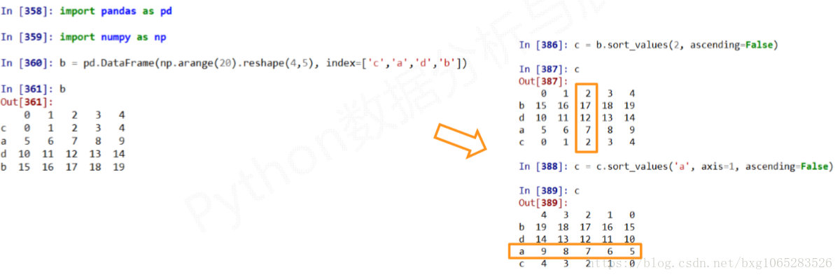
.sort_values()方法在指定轴上根据数值进行排序,默认升序
Series.sort_values(axis=0, ascending=True)
DataFrame.sort_values(by, axis=0, ascending=True)
import pandas as pd
import numpy as np
b=pd.DataFrame(np.arange(20).reshape(4,5),
               index=['c','a','d','b'])
print(b)
#     0   1   2   3   4
# c   0   1   2   3   4
# a   5   6   7   8   9
# d  10  11  12  13  14
# b  15  16  17  18  19
c=b.sort_values(2,ascending=False)
#     0   1   2   3   4
# b  15  16  17  18  19
# d  10  11  12  13  14
# a   5   6   7   8   9
# c   0   1   2   3   4
print(c)
c=c.sort_values('a',axis=1,ascending=False)
print(c)
#     4   3   2   1   0
# b  19  18  17  16  15
# d  14  13  12  11  10
# a   9   8   7   6   5
# c   4   3   2   1   0
NaN统一放到排序末尾
扫描二维码关注公众号,回复:
145431 查看本文章

import pandas as pd
import numpy as np
a=pd.DataFrame(np.arange(12).reshape(3,4),index=['a','b','c'])
print(a)
#    0  1   2   3
# a  0  1   2   3
# b  4  5   6   7
# c  8  9  10  11
b=pd.DataFrame(np.arange(20).reshape(4,5),
                index=['c','a','d','b'])
print(b)
#     0   1   2   3   4
# c   0   1   2   3   4
# a   5   6   7   8   9
# d  10  11  12  13  14
# b  15  16  17  18  19
c=a+b
print(c)
#       0     1     2     3   4
# a   5.0   7.0   9.0  11.0 NaN
# b  19.0  21.0  23.0  25.0 NaN
# c   8.0  10.0  12.0  14.0 NaN
# d   NaN   NaN   NaN   NaN NaN
print(c.sort_values(2,ascending=False))
#      0     1     2     3   4
# b  19.0  21.0  23.0  25.0 NaN
# c   8.0  10.0  12.0  14.0 NaN
# a   5.0   7.0   9.0  11.0 NaN
# d   NaN   NaN   NaN   NaN NaN
print(c.sort_values(2,ascending=True))
#       0     1     2     3   4
# a   5.0   7.0   9.0  11.0 NaN
# c   8.0  10.0  12.0  14.0 NaN
# b  19.0  21.0  23.0  25.0 NaN
# d   NaN   NaN   NaN   NaN NaN
2.数据的基本统计分析

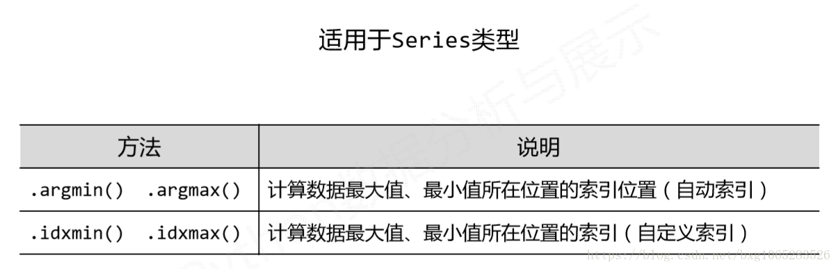
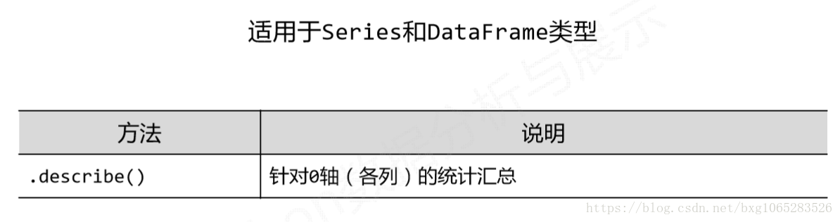
import pandas as pd
import numpy as np
a=pd.Series([9,8,7,6],index=['a','b','c','d'])
print(a)
# a    9
# b    8
# c    7
# d    6
# dtype: int64
print(a.describe())
# count    4.000000
# mean     7.500000
# std      1.290994
# min      6.000000
# 25%      6.750000
# 50%      7.500000
# 75%      8.250000
# max      9.000000
# dtype: float64
print(type(a.describe()))
# <class 'pandas.core.series.Series'>
print(a.describe()['count'])
# 4.0
print(a.describe()['max'])
# 9.0
b=pd.DataFrame(np.arange(20).reshape(4,5),
                index=['c','a','d','b'])
print(b.describe())
#                0          1          2          3          4
# count   4.000000   4.000000   4.000000   4.000000   4.000000
# mean    7.500000   8.500000   9.500000  10.500000  11.500000
# std     6.454972   6.454972   6.454972   6.454972   6.454972
# min     0.000000   1.000000   2.000000   3.000000   4.000000
# 25%     3.750000   4.750000   5.750000   6.750000   7.750000
# 50%     7.500000   8.500000   9.500000  10.500000  11.500000
# 75%    11.250000  12.250000  13.250000  14.250000  15.250000
# max    15.000000  16.000000  17.000000  18.000000  19.000000
print(type(b.describe()))
# <class 'pandas.core.frame.DataFrame'>
print(b.describe()[2])
# count     4.000000
# mean      9.500000
# std       6.454972
# min       2.000000
# 25%       5.750000
# 50%       9.500000
# 75%      13.250000
# max      17.000000
# Name: 2, dtype: float64
3.数据的累计统计分析
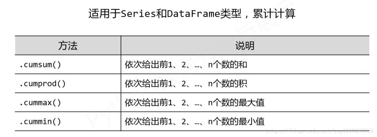
import pandas as pd
import numpy as np
b=pd.DataFrame(np.arange(20).reshape(4,5),
                index=['c','a','d','b'])
print(b)
#     0   1   2   3   4
# c   0   1   2   3   4
# a   5   6   7   8   9
# d  10  11  12  13  14
# b  15  16  17  18  19
print(b.cumsum())
#     0   1   2   3   4
# c   0   1   2   3   4
# a   5   7   9  11  13
# d  15  18  21  24  27
# b  30  34  38  42  46
print(b.cumprod())
#    0     1     2     3     4
# c  0     1     2     3     4
# a  0     6    14    24    36
# d  0    66   168   312   504
# b  0  1056  2856  5616  9576
print(b.cummin())
#    0  1  2  3  4
# c  0  1  2  3  4
# a  0  1  2  3  4
# d  0  1  2  3  4
# b  0  1  2  3  4
print(b.cummax())
#     0   1   2   3   4
# c   0   1   2   3   4
# a   5   6   7   8   9
# d  10  11  12  13  14
# b  15  16  17  18  19
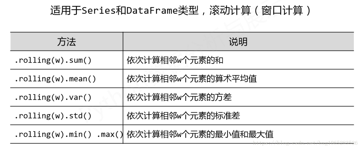
import pandas as pd
import numpy as np
b=pd.DataFrame(np.arange(20).reshape(4,5),
                index=['c','a','d','b'])
print(b)
#     0   1   2   3   4
# c   0   1   2   3   4
# a   5   6   7   8   9
# d  10  11  12  13  14
# b  15  16  17  18  19
print(b.rolling(2).sum())
#       0     1     2     3     4
# c   NaN   NaN   NaN   NaN   NaN
# a   5.0   7.0   9.0  11.0  13.0
# d  15.0  17.0  19.0  21.0  23.0
# b  25.0  27.0  29.0  31.0  33.0
print(b.rolling(3).sum())
#       0     1     2     3     4
# c   NaN   NaN   NaN   NaN   NaN
# a   NaN   NaN   NaN   NaN   NaN
# d  15.0  18.0  21.0  24.0  27.0
# b  30.0  33.0  36.0  39.0  42.0
5.数据的相关分析
相关性:
•X增大,Y增大,两个变量正相关
•X增大,Y减小,两个变量负相关
•X增大,Y无视,两个变量不相关
协方差:

•协方差>0, X和Y正相关
•协方差<0, X和Y负相关
•协方差=0, X和Y独立无关
Person相关系数:r取值范围[‐1,1]

•0.8‐1.0 极强相关
•0.6‐0.8 强相关
•0.4‐0.6 中等程度相关
•0.2‐0.4 弱相关
•0.0‐0.2 极弱相关或无相关

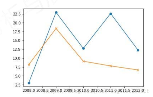
实例:
import pandas as pd
import numpy as np
hprice=pd.Series([3.04,22.93,12.75,22.6,12.33],
                 index=['2008','2009','2010','2011','2012'])
m2=pd.Series([8.18,18.38,9.13,7.82,6.69],
             index=['2008','2009','2010','2011','2012'])
print(hprice.corr(m2))
#0.5239439145220387