Opencv之边缘检测卷积算子(roberts与prewitt)

学习资料参考：

张平.《OpenCV算法精解：基于Python与C++》.[Z].北京.电子工业出版社.2017.

---

Roberts算子

原理

使用Roberts进行边缘检测，也就是使用以下两个卷积核与图像进行分别卷积。(图中阴影部分数值为锚点所在)

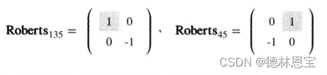
注意在实际讨论中一般将相近两点的函数值差值作为斜率。如

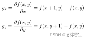
那么上述的两个卷积核也就好理解了。类似于
f(x,y) - f(x + 1,y + 1)与f(x,y) - f(x - 1,y + 1)两个函数差值。

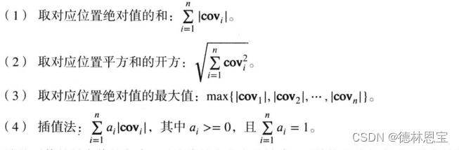
在边缘我们知道，边缘处的像素差值较大，斜率较大。那么下列给出四种衡量标准：

程序实现

import numpy as np
import cv2
from scipy import signal


def roberts(I, _boundary='fill', _fillvalue=0):
    # 图像的高和宽
    H1, W1 = I.shape
    # 卷积核的大小
    H2, W2 = 2, 2
    # 卷积核1以及锚点位置
    R1 = np.array([[1, 0], [0, -1]], np.float32)
    kr1, kc1 = 0, 0
    # 计算full卷积
    IconR1 = signal.convolve2d(I, R1, mode='full', boundary=_boundary, fillvalue=_fillvalue)
    IconR1 = IconR1[H2 - kr1 - 1:H1 + H2 - kr1 - 1, W2 - kc1 - 1:W1 + W2 - kc1 - 1]
    # 卷积核2
    R2 = np.array([[0, 1], [-1, 0]], np.float32)
    # 先计算full卷积
    IconR2 = signal.convolve2d(I, R2, mode='full', boundary=_boundary, fillvalue=_fillvalue)
    # 锚点的位置
    kr2, kc2 = 0, 1
    # 根据锚点的位置截取full卷积，从而得到same卷积
    IconR2 = IconR2[H2 - kr2 - 1:H1 + H2 - kr2 - 1, W2 - kc2 - 1:W1 + W2 - kc2 - 1]
    return IconR1, IconR2


if __name__ == "__main__":
    image = cv2.imread(r"C:\Users\1\Pictures\test.jpg", 0)
    cv2.imshow("imgae", image)
    # 卷积，边界扩充采用symm
    IconR1, IconR2 = roberts(image, 'symm')
    # 45度方向上的边缘强度的灰度级显示
    IconR1 = np.abs(IconR1)
    edge_45 = IconR1.astype(np.uint8)
    cv2.imshow("edge_45", edge_45)
    # 135度方向上的边缘强度
    IconR2 = np.abs(IconR2)
    edge_135 = IconR2.astype(np.uint8)
    cv2.imshow("edge_135", edge_135)
    # 用平方和的开方来衡量最后输出的边缘
    edge = np.sqrt(np.power(IconR1, 2.0) + np.power(IconR2, 2.0))
    edge = np.round(edge)
    edge[edge > 255] = 255
    edge = edge.astype(np.uint8)
    # 显示边缘
    cv2.imshow("edge", edge)
    cv2.waitKey(0)
    cv2.destroyAllWindows()

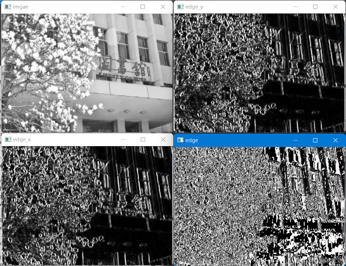
运行结果

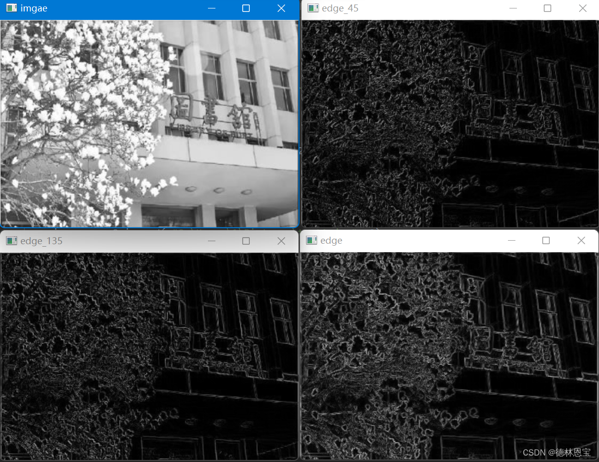
综合分析输出图片可知，在edge45与edge135上，轮廓较明显分别在45度方向与135度方向，而edge是两者的综合。

---

Prewitt算子

原理

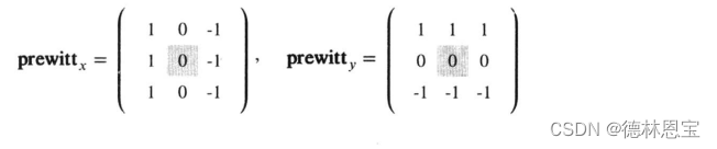
与Roberts算子类似，prewitt算子也是两个卷积核。（并且其中带阴影部分的数字是锚点所在）

并且发现上述两个矩阵是可以进行分离的，如下所示

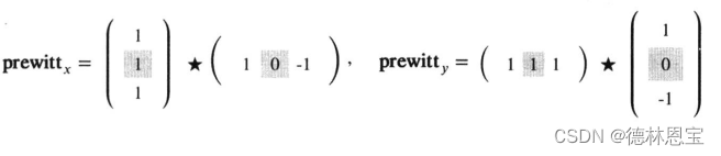
根据分离的结果可知，$prewit{t}_x$算子的卷积可以分为先进行垂直方向的均值平滑，然后进行水平方向的差分。同理，$prewit{t}_y$也可类似进行理解。

程序实现

import numpy as np
import cv2
from scipy import signal


def prewitt(I, _boundary='symm'):
    # prewitt_x卷积运算
    # 垂直方向的均值平滑
    ones_y = np.array([[1], [1], [1]], np.float32)
    i_conv_pre_x = signal.convolve2d(I, ones_y, mode='same', boundary=_boundary)
    # 水平方向的差分
    diff_x = np.array([[1, 0, -1]], np.float32)
    i_conv_pre_x = signal.convolve2d(i_conv_pre_x, diff_x, mode='same', boundary=_boundary)
    # prewitt_y卷积运算
    # 水平方向的均值平滑
    ones_x = np.array([[1], [1], [1]], np.float32)
    i_conv_pre_y = signal.convolve2d(I, ones_x, mode='same', boundary=_boundary)
    # 垂直方向的差分
    diff_y = np.array([[1, 0, -1]], np.float32)
    i_conv_pre_y = signal.convolve2d(i_conv_pre_y, diff_y, mode='same', boundary=_boundary)
    return i_conv_pre_x, i_conv_pre_y


if __name__ == "__main__":
    image = cv2.imread(r"C:\Users\1\Pictures\test1.jpg", 0)
    cv2.imshow("imgae", image)
    # 卷积，边界扩充采用symm
    i_conv_pre_x, i_conv_pre_y = prewitt(image)
    # 取绝对值
    abs_i_conv_pre_x = np.abs(i_conv_pre_x)
    abs_i_conv_pre_y = np.abs(i_conv_pre_y)
    # 边缘强度的灰度值显示
    edge_x = abs_i_conv_pre_x.copy()
    edge_y = abs_i_conv_pre_y.copy()
    # 截断
    edge_x[edge_x > 255] = 255
    edge_y[edge_y > 255] = 255
    # 类型转换
    edge_x = edge_x.astype(np.uint8)
    edge_y = edge_y.astype(np.uint8)
    cv2.imshow("edge_x", edge_x)
    cv2.imshow("edge_y", edge_y)
    # 求解边缘强度
    edge = 0.5 * i_conv_pre_x + 0.5 * i_conv_pre_y
    edge[edge > 255] = 255
    # 显示边缘
    edge = edge.astype(np.uint8)
    cv2.imshow("edge", edge)
    cv2.waitKey(0)
    cv2.destroyAllWindows()

运行结果

---