Opencv之高斯拉普拉斯边缘检测

学习资料参考：

张平.《OpenCV算法精解：基于Python与C++》.[Z].北京.电子工业出版社.2017.

---

前言

我们知道在进行拉普拉斯边缘检测时，并没有对图像进行平滑处理，就会对噪声产生明显的响应（可以进行对比实验查看效果）。那么，我们在使用拉普拉斯进行边缘检测时，首先要对图像进行高斯平滑处理，然后再进行拉普拉斯与图像的卷积操作。那么这就需要进行两次卷积运算。而为了将卷积次数控制在一次，聪明的人们发现可以借助二维高斯函数（如下图所示）进行拉普拉斯变换。(真的很佩服这些数学家们！)

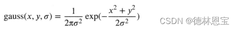
我从opencv书上截取推导过程如下所示：

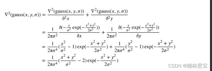
上述得出的最终结果被称为高斯拉普拉斯。

---

检测原理

1. 构建窗口大小为$H\ast W$、标准差为$\sigma$的高斯拉普拉斯卷积核。
   
   其中$H$与$W$均是奇数，并且$H=W$,卷积核的锚点在$((H-1)/2,(W-1)/2)$处。
2. 然后使用上面构建的卷积核，进行卷积。
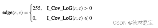
3. 边缘二值化显示，与Laplace的二值化一样。
   

---

python实现

import numpy as np
from scipy import signal
import cv2


def createLoGKernel(sigma, size):
    H, W = size
    r, c = np.mgrid[0:H:1, 0:W:1]
    r -= (H - 1) // 2
    c -= (W - 1) // 2
    sigma2 = pow(sigma, 2.0)
    norm2 = np.power(r, 2.0) + np.power(c, 2.0)
    LoGKernel = (norm2 / sigma2 - 2) * np.exp(-norm2 / (2 * sigma2))
    return LoGKernel


def LoG(image, sigma, size, _boundary='symm'):
    loGKernel = createLoGKernel(sigma, size)
    img_conv_log = signal.convolve2d(image, loGKernel, 'same', boundary=_boundary)
    return img_conv_log


if __name__ == "__main__":
    image = cv2.imread(r"C:\Users\1\Pictures\test1.jpg", 0)
    cv2.imshow("原图", image)
    img_conv_log = LoG(image, 2, (13, 13), 'symm')
    edge_binary = np.copy(img_conv_log)
    edge_binary[edge_binary > 0] = 255
    edge_binary[edge_binary <= 0] = 0
    edge_binary = edge_binary.astype(np.uint8)
    cv2.imshow("edge_binary", edge_binary)
    cv2.waitKey(0)
    cv2.destroyAllWindows()

运行结果

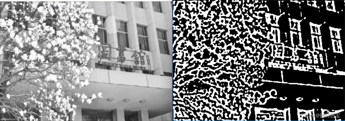
注意，经过测试发现，标准差越大，图像在边缘上的失真越严重。对于高斯拉普拉斯核的尺寸，一般取$(6\ast \sigma +1)\ast (6\ast \sigma +1)$.