声明:内容非原创,是学习内容的总结,版权所属姜老师
线性回归引入
# 线性回归导入
from sklearn.linear_model import LinearRegression
from sklearn.neighbors import KNeighborsRegressor
import numpy as np
import pandas as pd
from pandas import Series,DataFrame

import matplotlib.pyplot as plt
%matplotlib inline
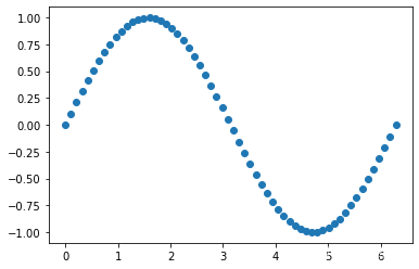
# 生成一组假数据 假设x和y都遵循正弦分布
x = np.linspace(0, 2*np.pi, 60)
y = np.sin(x)
plt.scatter(x,y)
<matplotlib.collections.PathCollection at 0x1facb5abdc0>
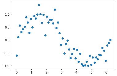
# 生成噪声数据 (-0.5, 0.5)
bias = np.random.random(30) - 0.5
bias
array([-0.39502105,  0.24340303,  0.08361402, -0.00268972, -0.03143423,
       -0.41971947,  0.2567082 , -0.07361341, -0.14754526, -0.41319023,
        0.21895744, -0.31080432,  0.21599872, -0.08704963, -0.1380524 ,
       -0.23046208,  0.3592808 , -0.16425466, -0.00648164,  0.24217655,
        0.43796813,  0.21696034,  0.4143489 ,  0.22052109,  0.25845568,
       -0.35609606, -0.00906317, -0.24740159, -0.21426299, -0.13506899])
# 把噪声数据添加到y中
y[::2] += bias
plt.scatter(x,y)
<matplotlib.collections.PathCollection at 0x1facc2489a0>
x.shape
(60,)
# vsm 映射
X = x.reshape(-1,1)
X.shape
(60, 1)
X
array([[0.        ],
       [0.10649467],
       [0.21298933],
       [0.319484  ],
       [0.42597866],
       [0.53247333],
       [0.638968  ],
       [0.74546266],
       [0.85195733],
       [0.958452  ],
       [1.06494666],
       [1.17144133],
       [1.27793599],
       [1.38443066],
       [1.49092533],
       [1.59741999],
       [1.70391466],
       [1.81040933],
       [1.91690399],
       [2.02339866],
       [2.12989332],
       [2.23638799],
       [2.34288266],
       [2.44937732],
       [2.55587199],
       [2.66236666],
       [2.76886132],
       [2.87535599],
       [2.98185065],
       [3.08834532],
       [3.19483999],
       [3.30133465],
       [3.40782932],
       [3.51432399],
       [3.62081865],
       [3.72731332],
       [3.83380798],
       [3.94030265],
       [4.04679732],
       [4.15329198],
       [4.25978665],
       [4.36628132],
       [4.47277598],
       [4.57927065],
       [4.68576531],
       [4.79225998],
       [4.89875465],
       [5.00524931],
       [5.11174398],
       [5.21823864],
       [5.32473331],
       [5.43122798],
       [5.53772264],
       [5.64421731],
       [5.75071198],
       [5.85720664],
       [5.96370131],
       [6.07019597],
       [6.17669064],
       [6.28318531]])
# 1. knn实例化
knn =KNeighborsRegressor(n_neighbors=3)
# 2. 训练fit 实例化好的knn回归器
knn.fit(X, y)
KNeighborsRegressor(n_neighbors=3)
# 生成测试数据,别忘了和X同样的结构
# 注意,生成的数据只要不是60就行, 因为我们样本集数据也是同样范围的等差计算出来的
X_test = np.linspace(0, 2*np.pi, 45).reshape(-1,1)
X_test
array([[0.        ],
       [0.14279967],
       [0.28559933],
       [0.428399  ],
       [0.57119866],
       [0.71399833],
       [0.856798  ],
       [0.99959766],
       [1.14239733],
       [1.28519699],
       [1.42799666],
       [1.57079633],
       [1.71359599],
       [1.85639566],
       [1.99919533],
       [2.14199499],
       [2.28479466],
       [2.42759432],
       [2.57039399],
       [2.71319366],
       [2.85599332],
       [2.99879299],
       [3.14159265],
       [3.28439232],
       [3.42719199],
       [3.56999165],
       [3.71279132],
       [3.85559098],
       [3.99839065],
       [4.14119032],
       [4.28398998],
       [4.42678965],
       [4.56958931],
       [4.71238898],
       [4.85518865],
       [4.99798831],
       [5.14078798],
       [5.28358764],
       [5.42638731],
       [5.56918698],
       [5.71198664],
       [5.85478631],
       [5.99758598],
       [6.14038564],
       [6.28318531]])
# 3.预测:使用X_test作为特征
y1_ = knn.predict(X_test)
y1_
array([ 0.01827837,  0.01827837,  0.42913475,  0.41198503,  0.60033228,
        0.61071011,  0.59043822,  0.52817234,  0.74745077,  0.91117407,
        1.05438104,  1.00544205,  0.87894106,  0.60410825,  0.58399583,
        0.78779728,  0.74957241,  0.86489298,  0.75704464,  0.76885007,
        0.24759279,  0.04078003, -0.21986071, -0.2357875 , -0.18423447,
       -0.53796589, -0.53252107, -0.53902763, -0.64776802, -0.58808059,
       -0.77527639, -0.9766071 , -0.94502224, -0.94463684, -0.85647279,
       -0.75180678, -0.83833303, -0.76975748, -0.66825555, -0.6397318 ,
       -0.43908767, -0.50822301, -0.47612273, -0.11130414, -0.11130414])
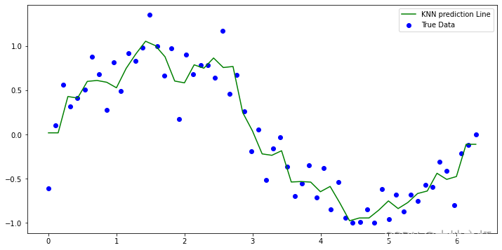
# 绘制 knn回归的预测结果
plt.figure(figsize=(12,6))
plt.scatter(x, y ,label='True Data', color ='blue')
plt.plot(X_test,y1_, label='KNN prediction Line',color = 'green')
plt.legend()
plt.show()
# 使用线性回归做预测
# 1.实例化线性模型 linearRegression
linear = LinearRegression()
# 2.fit训练模型 给定x和y
linear.fit(X,y)
LinearRegression()
# 3.模型预测 利用X_test进行预测
y2_ = linear.predict(X_test)
y2_
array([ 8.35573602e-01,  7.97617275e-01,  7.59660948e-01,  7.21704620e-01,
        6.83748293e-01,  6.45791966e-01,  6.07835639e-01,  5.69879311e-01,
        5.31922984e-01,  4.93966657e-01,  4.56010330e-01,  4.18054002e-01,
        3.80097675e-01,  3.42141348e-01,  3.04185021e-01,  2.66228693e-01,
        2.28272366e-01,  1.90316039e-01,  1.52359712e-01,  1.14403384e-01,
        7.64470572e-02,  3.84907299e-02,  5.34402699e-04, -3.74219245e-02,
       -7.53782518e-02, -1.13334579e-01, -1.51290906e-01, -1.89247234e-01,
       -2.27203561e-01, -2.65159888e-01, -3.03116215e-01, -3.41072542e-01,
       -3.79028870e-01, -4.16985197e-01, -4.54941524e-01, -4.92897851e-01,
       -5.30854179e-01, -5.68810506e-01, -6.06766833e-01, -6.44723160e-01,
       -6.82679488e-01, -7.20635815e-01, -7.58592142e-01, -7.96548469e-01,
       -8.34504797e-01])
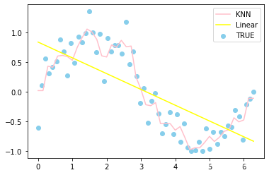
# 预测结果作一个绘制
plt.scatter(x,y,label='TRUE',color = 'skyblue')
plt.plot(X_test,y1_,label='KNN',color='pink')
plt.plot(X_test,y2_,label='Linear',color='yellow')
plt.legend()
plt.show()
knn线性回归(糖尿病数据集)
```python
import numpy as np
import pandas as pd
from pandas import Series,DataFrame

import matplotlib.pyplot as plt
import seaborn as sns
%matplotlib inline
from sklearn.linear_model import LinearRegression
from sklearn.neighbors import KNeighborsRegressor
from sklearn.datasets import load_diabetes
# 这个是diabetes糖尿病数据集
diabetes = load_diabetes()
diabetes
{'data': array([[ 0.03807591,  0.05068012,  0.06169621, ..., -0.00259226,
          0.01990842, -0.01764613],
        [-0.00188202, -0.04464164, -0.05147406, ..., -0.03949338,
         -0.06832974, -0.09220405],
        [ 0.08529891,  0.05068012,  0.04445121, ..., -0.00259226,
          0.00286377, -0.02593034],
        ...,
        [ 0.04170844,  0.05068012, -0.01590626, ..., -0.01107952,
         -0.04687948,  0.01549073],
        [-0.04547248, -0.04464164,  0.03906215, ...,  0.02655962,
          0.04452837, -0.02593034],
        [-0.04547248, -0.04464164, -0.0730303 , ..., -0.03949338,
         -0.00421986,  0.00306441]]),
 'target': array([151.,  75., 141., 206., 135.,  97., 138.,  63., 110., 310., 101.,
         69., 179., 185., 118., 171., 166., 144.,  97., 168.,  68.,  49.,
         68., 245., 184., 202., 137.,  85., 131., 283., 129.,  59., 341.,
         87.,  65., 102., 265., 276., 252.,  90., 100.,  55.,  61.,  92.,
        259.,  53., 190., 142.,  75., 142., 155., 225.,  59., 104., 182.,
        128.,  52.,  37., 170., 170.,  61., 144.,  52., 128.,  71., 163.,
        150.,  97., 160., 178.,  48., 270., 202., 111.,  85.,  42., 170.,
        200., 252., 113., 143.,  51.,  52., 210.,  65., 141.,  55., 134.,
         42., 111.,  98., 164.,  48.,  96.,  90., 162., 150., 279.,  92.,
         83., 128., 102., 302., 198.,  95.,  53., 134., 144., 232.,  81.,
        104.,  59., 246., 297., 258., 229., 275., 281., 179., 200., 200.,
        173., 180.,  84., 121., 161.,  99., 109., 115., 268., 274., 158.,
        107.,  83., 103., 272.,  85., 280., 336., 281., 118., 317., 235.,
         60., 174., 259., 178., 128.,  96., 126., 288.,  88., 292.,  71.,
        197., 186.,  25.,  84.,  96., 195.,  53., 217., 172., 131., 214.,
         59.,  70., 220., 268., 152.,  47.,  74., 295., 101., 151., 127.,
        237., 225.,  81., 151., 107.,  64., 138., 185., 265., 101., 137.,
        143., 141.,  79., 292., 178.,  91., 116.,  86., 122.,  72., 129.,
        142.,  90., 158.,  39., 196., 222., 277.,  99., 196., 202., 155.,
         77., 191.,  70.,  73.,  49.,  65., 263., 248., 296., 214., 185.,
         78.,  93., 252., 150.,  77., 208.,  77., 108., 160.,  53., 220.,
        154., 259.,  90., 246., 124.,  67.,  72., 257., 262., 275., 177.,
         71.,  47., 187., 125.,  78.,  51., 258., 215., 303., 243.,  91.,
        150., 310., 153., 346.,  63.,  89.,  50.,  39., 103., 308., 116.,
        145.,  74.,  45., 115., 264.,  87., 202., 127., 182., 241.,  66.,
         94., 283.,  64., 102., 200., 265.,  94., 230., 181., 156., 233.,
         60., 219.,  80.,  68., 332., 248.,  84., 200.,  55.,  85.,  89.,
         31., 129.,  83., 275.,  65., 198., 236., 253., 124.,  44., 172.,
        114., 142., 109., 180., 144., 163., 147.,  97., 220., 190., 109.,
        191., 122., 230., 242., 248., 249., 192., 131., 237.,  78., 135.,
        244., 199., 270., 164.,  72.,  96., 306.,  91., 214.,  95., 216.,
        263., 178., 113., 200., 139., 139.,  88., 148.,  88., 243.,  71.,
         77., 109., 272.,  60.,  54., 221.,  90., 311., 281., 182., 321.,
         58., 262., 206., 233., 242., 123., 167.,  63., 197.,  71., 168.,
        140., 217., 121., 235., 245.,  40.,  52., 104., 132.,  88.,  69.,
        219.,  72., 201., 110.,  51., 277.,  63., 118.,  69., 273., 258.,
         43., 198., 242., 232., 175.,  93., 168., 275., 293., 281.,  72.,
        140., 189., 181., 209., 136., 261., 113., 131., 174., 257.,  55.,
         84.,  42., 146., 212., 233.,  91., 111., 152., 120.,  67., 310.,
         94., 183.,  66., 173.,  72.,  49.,  64.,  48., 178., 104., 132.,
        220.,  57.]),
 'frame': None,
 'DESCR': '.. _diabetes_dataset:\n\nDiabetes dataset\n----------------\n\nTen baseline variables, age, sex, body mass index, average blood\npressure, and six blood serum measurements were obtained for each of n =\n442 diabetes patients, as well as the response of interest, a\nquantitative measure of disease progression one year after baseline.\n\n**Data Set Characteristics:**\n\n  :Number of Instances: 442\n\n  :Number of Attributes: First 10 columns are numeric predictive values\n\n  :Target: Column 11 is a quantitative measure of disease progression one year after baseline\n\n  :Attribute Information:\n      - age     age in years\n      - sex\n      - bmi     body mass index\n      - bp      average blood pressure\n      - s1      tc, total serum cholesterol\n      - s2      ldl, low-density lipoproteins\n      - s3      hdl, high-density lipoproteins\n      - s4      tch, total cholesterol / HDL\n      - s5      ltg, possibly log of serum triglycerides level\n      - s6      glu, blood sugar level\n\nNote: Each of these 10 feature variables have been mean centered and scaled by the standard deviation times `n_samples` (i.e. the sum of squares of each column totals 1).\n\nSource URL:\nhttps://www4.stat.ncsu.edu/~boos/var.select/diabetes.html\n\nFor more information see:\nBradley Efron, Trevor Hastie, Iain Johnstone and Robert Tibshirani (2004) "Least Angle Regression," Annals of Statistics (with discussion), 407-499.\n(https://web.stanford.edu/~hastie/Papers/LARS/LeastAngle_2002.pdf)',
 'feature_names': ['age',
  'sex',
  'bmi',
  'bp',
  's1',
  's2',
  's3',
  's4',
  's5',
  's6'],
 'data_filename': 'D:\\software\\anaconda\\lib\\site-packages\\sklearn\\datasets\\data\\diabetes_data.csv.gz',
 'target_filename': 'D:\\software\\anaconda\\lib\\site-packages\\sklearn\\datasets\\data\\diabetes_target.csv.gz'}
print(diabetes.DESCR)
.. _diabetes_dataset:

Diabetes dataset
----------------

Ten baseline variables, age, sex, body mass index, average blood
pressure, and six blood serum measurements were obtained for each of n =
442 diabetes patients, as well as the response of interest, a
quantitative measure of disease progression one year after baseline.

**Data Set Characteristics:**

  :Number of Instances: 442

  :Number of Attributes: First 10 columns are numeric predictive values

  :Target: Column 11 is a quantitative measure of disease progression one year after baseline

  :Attribute Information:
      - age     age in years
      - sex
      - bmi     body mass index
      - bp      average blood pressure
      - s1      tc, total serum cholesterol
      - s2      ldl, low-density lipoproteins
      - s3      hdl, high-density lipoproteins
      - s4      tch, total cholesterol / HDL
      - s5      ltg, possibly log of serum triglycerides level
      - s6      glu, blood sugar level

Note: Each of these 10 feature variables have been mean centered and scaled by the standard deviation times `n_samples` (i.e. the sum of squares of each column totals 1).

Source URL:
https://www4.stat.ncsu.edu/~boos/var.select/diabetes.html

For more information see:
Bradley Efron, Trevor Hastie, Iain Johnstone and Robert Tibshirani (2004) "Least Angle Regression," Annals of Statistics (with discussion), 407-499.
(https://web.stanford.edu/~hastie/Papers/LARS/LeastAngle_2002.pdf)
diabetes.feature_names
['age', 'sex', 'bmi', 'bp', 's1', 's2', 's3', 's4', 's5', 's6']
# 导出数据成为DataFrame
dataSets = DataFrame(data=diabetes.data,columns=diabetes.feature_names)
dataSets.head()
| age | sex | bmi | bp | s1 | s2 | s3 | s4 | s5 | s6 | |
|---|---|---|---|---|---|---|---|---|---|---|
| 0 | 0.038076 | 0.050680 | 0.061696 | 0.021872 | -0.044223 | -0.034821 | -0.043401 | -0.002592 | 0.019908 | -0.017646 |
| 1 | -0.001882 | -0.044642 | -0.051474 | -0.026328 | -0.008449 | -0.019163 | 0.074412 | -0.039493 | -0.068330 | -0.092204 |
| 2 | 0.085299 | 0.050680 | 0.044451 | -0.005671 | -0.045599 | -0.034194 | -0.032356 | -0.002592 | 0.002864 | -0.025930 |
| 3 | -0.089063 | -0.044642 | -0.011595 | -0.036656 | 0.012191 | 0.024991 | -0.036038 | 0.034309 | 0.022692 | -0.009362 |
| 4 | 0.005383 | -0.044642 | -0.036385 | 0.021872 | 0.003935 | 0.015596 | 0.008142 | -0.002592 | -0.031991 | -0.046641 |
dataSets.describe().T
| count | mean | std | min | 25% | 50% | 75% | max | |
|---|---|---|---|---|---|---|---|---|
| age | 442.0 | -3.634285e-16 | 0.047619 | -0.107226 | -0.037299 | 0.005383 | 0.038076 | 0.110727 |
| sex | 442.0 | 1.308343e-16 | 0.047619 | -0.044642 | -0.044642 | -0.044642 | 0.050680 | 0.050680 |
| bmi | 442.0 | -8.045349e-16 | 0.047619 | -0.090275 | -0.034229 | -0.007284 | 0.031248 | 0.170555 |
| bp | 442.0 | 1.281655e-16 | 0.047619 | -0.112400 | -0.036656 | -0.005671 | 0.035644 | 0.132044 |
| s1 | 442.0 | -8.835316e-17 | 0.047619 | -0.126781 | -0.034248 | -0.004321 | 0.028358 | 0.153914 |
| s2 | 442.0 | 1.327024e-16 | 0.047619 | -0.115613 | -0.030358 | -0.003819 | 0.029844 | 0.198788 |
| s3 | 442.0 | -4.574646e-16 | 0.047619 | -0.102307 | -0.035117 | -0.006584 | 0.029312 | 0.181179 |
| s4 | 442.0 | 3.777301e-16 | 0.047619 | -0.076395 | -0.039493 | -0.002592 | 0.034309 | 0.185234 |
| s5 | 442.0 | -3.830854e-16 | 0.047619 | -0.126097 | -0.033249 | -0.001948 | 0.032433 | 0.133599 |
| s6 | 442.0 | -3.412882e-16 | 0.047619 | -0.137767 | -0.033179 | -0.001078 | 0.027917 | 0.135612 |
# 样本集拆分
from sklearn.model_selection import train_test_split
# 标签拿进来
target = diabetes.target
# 拆分训练集测试集
X_train,X_test,y_train,y_test = train_test_split(dataSets, target,test_size=0.2, random_state=2)
# 1.实例化模型 knn
knn = KNeighborsRegressor()
# 2.训练模型fit
knn.fit(X_train,y_train)
KNeighborsRegressor()
# MAE MSE
from sklearn.metrics import mean_squared_error, mean_absolute_error
# 泛化误差 -mse
mean_squared_error(y_test, knn.predict(X_test))
3941.039550561798
# 平均绝对误差  mae
mean_absolute_error(y_test, knn.predict(X_test))
50.06966292134831
target
array([151.,  75., 141., 206., 135.,  97., 138.,  63., 110., 310., 101.,
        69., 179., 185., 118., 171., 166., 144.,  97., 168.,  68.,  49.,
        68., 245., 184., 202., 137.,  85., 131., 283., 129.,  59., 341.,
        87.,  65., 102., 265., 276., 252.,  90., 100.,  55.,  61.,  92.,
       259.,  53., 190., 142.,  75., 142., 155., 225.,  59., 104., 182.,
       128.,  52.,  37., 170., 170.,  61., 144.,  52., 128.,  71., 163.,
       150.,  97., 160., 178.,  48., 270., 202., 111.,  85.,  42., 170.,
       200., 252., 113., 143.,  51.,  52., 210.,  65., 141.,  55., 134.,
        42., 111.,  98., 164.,  48.,  96.,  90., 162., 150., 279.,  92.,
        83., 128., 102., 302., 198.,  95.,  53., 134., 144., 232.,  81.,
       104.,  59., 246., 297., 258., 229., 275., 281., 179., 200., 200.,
       173., 180.,  84., 121., 161.,  99., 109., 115., 268., 274., 158.,
       107.,  83., 103., 272.,  85., 280., 336., 281., 118., 317., 235.,
        60., 174., 259., 178., 128.,  96., 126., 288.,  88., 292.,  71.,
       197., 186.,  25.,  84.,  96., 195.,  53., 217., 172., 131., 214.,
        59.,  70., 220., 268., 152.,  47.,  74., 295., 101., 151., 127.,
       237., 225.,  81., 151., 107.,  64., 138., 185., 265., 101., 137.,
       143., 141.,  79., 292., 178.,  91., 116.,  86., 122.,  72., 129.,
       142.,  90., 158.,  39., 196., 222., 277.,  99., 196., 202., 155.,
        77., 191.,  70.,  73.,  49.,  65., 263., 248., 296., 214., 185.,
        78.,  93., 252., 150.,  77., 208.,  77., 108., 160.,  53., 220.,
       154., 259.,  90., 246., 124.,  67.,  72., 257., 262., 275., 177.,
        71.,  47., 187., 125.,  78.,  51., 258., 215., 303., 243.,  91.,
       150., 310., 153., 346.,  63.,  89.,  50.,  39., 103., 308., 116.,
       145.,  74.,  45., 115., 264.,  87., 202., 127., 182., 241.,  66.,
        94., 283.,  64., 102., 200., 265.,  94., 230., 181., 156., 233.,
        60., 219.,  80.,  68., 332., 248.,  84., 200.,  55.,  85.,  89.,
        31., 129.,  83., 275.,  65., 198., 236., 253., 124.,  44., 172.,
       114., 142., 109., 180., 144., 163., 147.,  97., 220., 190., 109.,
       191., 122., 230., 242., 248., 249., 192., 131., 237.,  78., 135.,
       244., 199., 270., 164.,  72.,  96., 306.,  91., 214.,  95., 216.,
       263., 178., 113., 200., 139., 139.,  88., 148.,  88., 243.,  71.,
        77., 109., 272.,  60.,  54., 221.,  90., 311., 281., 182., 321.,
        58., 262., 206., 233., 242., 123., 167.,  63., 197.,  71., 168.,
       140., 217., 121., 235., 245.,  40.,  52., 104., 132.,  88.,  69.,
       219.,  72., 201., 110.,  51., 277.,  63., 118.,  69., 273., 258.,
        43., 198., 242., 232., 175.,  93., 168., 275., 293., 281.,  72.,
       140., 189., 181., 209., 136., 261., 113., 131., 174., 257.,  55.,
        84.,  42., 146., 212., 233.,  91., 111., 152., 120.,  67., 310.,
        94., 183.,  66., 173.,  72.,  49.,  64.,  48., 178., 104., 132.,
       220.,  57.])
# 消除数据的量级(量纲)
# 1. 标准化 Z-SCORE StanderdScaller  - 均值为0 标准差为1
# 2. 区缩放 MinMaxScaller 缩放到[0,1]
from sklearn.preprocessing import StandardScaler, MinMaxScaler
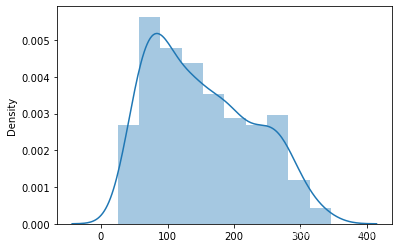
# 首先 查看target的数据分布
sns.distplot(target)
<AxesSubplot:ylabel='Density'>
# 1. 实例化
ss = StandardScaler()
# 2. 转化
ss_target = ss.fit_transform(target.reshape(-1,1))
ss_target
array([[-1.47194752e-02],
       [-1.00165882e+00],
       [-1.44579915e-01],
       [ 6.99512942e-01],
       [-2.22496178e-01],
       [-7.15965848e-01],
       [-1.83538046e-01],
       [-1.15749134e+00],
       [-5.47147277e-01],
       [ 2.05006151e+00],
     ......
       [-2.61454310e-01],
       [ 8.81317557e-01],
       [-1.23540761e+00]])
sns.distplot(ss_target)
<AxesSubplot:ylabel='Density'>
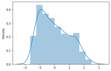
# 使用标准化之后的target 来建模(ss_target)
# 【注意】 random_state 要和之前的保持一致, 为的是保证两个模型使用的训练集和测试集一致
X_train, X_test, y_train, y_test = train_test_split(dataSets, ss_target, test_size=0.2, random_state=2)
# 重新训练k=5这个对象
knn.fit(X_train,y_train)
KNeighborsRegressor()
# 训练之后的新的评判
mean_squared_error(y_test,knn.predict(X_test))
0.6646064163260871
mean_absolute_error(y_test,knn.predict(X_test))
0.6502068430871709
找到一个更好的模型(knn调参,评价(MAE,MSE))
# 先试一下使用线性回归
#1.实例化
linear = LinearRegression()
#2.训
linear.fit(X_train,y_train)
#3.评判
mean_squared_error(y_test,linear.predict(X_test))
0.5218363683134858
问题:
- knn是可以调参的
- 算法评分是某一次的随机值
- 回归问题模型的好坏,要看泛化误差 和 经验误差
# 定义一个函数来评判模型
def cal_score(model, X,y, count, test_size):
    train_mse_list= []
    test_mse_list = []

    for i in range(count):
        X_train,X_test,y_train,y_test = train_test_split(X,y,test_size=test_size)
        model.fit(X,y)
        train_mse_list.append(mean_squared_error(y_train, model.predict(X_train)))
        test_mse_list.append(mean_squared_error(y_test, model.predict(X_test)))
    return np.array(train_mse_list),np.array(test_mse_list)
knn = KNeighborsRegressor(n_neighbors=5)
train_score_array,test_score_array = cal_score(model=knn,X=dataSets.values,y=target,count=10,test_size=0.3)
train_score_array.mean() ,train_score_array.std()
(2336.3235339805824, 87.16520782728838)
test_score_array.mean() ,test_score_array.std()
(2357.03569924812, 202.51164826039167)
linear = LinearRegression()
train_score_array,test_score_array = cal_score(model=linear,X=dataSets.values,y=target,count=10,test_size=0.3)
train_score_array.mean() ,train_score_array.std()
(2807.125616206974, 100.88450030074503)
test_score_array.mean() ,test_score_array.std()
(2981.8145928385716, 234.3857939318062)
# 评判一下 在不同的k值上的knn模型的表现
k_list = np.arange(1,21,2)

cols = []
for k in k_list:
    knn = KNeighborsRegressor(n_neighbors=k)
    train_scores,test_scores = cal_score(model=knn,X=dataSets.values,y=target,count=10,test_size=0.2)
    row = [k,
           train_scores.mean().tolist(),
           test_scores.mean().tolist(),
           train_scores.std().tolist(),
           test_scores.std().tolist()
    ]
    cols.append(row)
result= DataFrame(data=np.array(cols),columns=['k','Train_mean','Test_mean','Train_std','Test_std'])
result
| k | Train_mean | Test_mean | Train_std | Test_std | |
|---|---|---|---|---|---|
| 0 | 1.0 | 0.000000 | 0.000000 | 0.000000 | 0.000000 |
| 1 | 3.0 | 1937.297136 | 2021.645443 | 72.113122 | 286.021709 |
| 2 | 5.0 | 2333.390946 | 2378.906921 | 111.330407 | 441.568918 |
| 3 | 7.0 | 2635.195207 | 2542.229420 | 52.116173 | 206.707967 |
| 4 | 9.0 | 2731.609684 | 2615.471952 | 72.131433 | 286.094334 |
| 5 | 11.0 | 2724.262086 | 2998.797892 | 59.500027 | 235.994490 |
| 6 | 13.0 | 2829.240362 | 2869.213197 | 40.296168 | 159.826374 |
| 7 | 15.0 | 2794.546657 | 3125.196095 | 68.837757 | 273.030655 |
| 8 | 17.0 | 2898.627282 | 2875.761736 | 69.569247 | 275.931959 |
| 9 | 19.0 | 2868.687365 | 2924.798718 | 66.040720 | 261.936788 |
result.set_index('k').plot()
plt.xticks(result['k'].values)
plt.show()
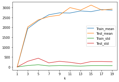
# 1.经验误差和泛化误差越接近并且越小
# 2. 经验误差和泛化误差的标准方差更小,越小越稳定


# 我们还能做什么?
# 还可以做特征处理。
# 理解数据
dataSets.describe().T
| count | mean | std | min | 25% | 50% | 75% | max | |
|---|---|---|---|---|---|---|---|---|
| age | 442.0 | -3.634285e-16 | 0.047619 | -0.107226 | -0.037299 | 0.005383 | 0.038076 | 0.110727 |
| sex | 442.0 | 1.308343e-16 | 0.047619 | -0.044642 | -0.044642 | -0.044642 | 0.050680 | 0.050680 |
| bmi | 442.0 | -8.045349e-16 | 0.047619 | -0.090275 | -0.034229 | -0.007284 | 0.031248 | 0.170555 |
| bp | 442.0 | 1.281655e-16 | 0.047619 | -0.112400 | -0.036656 | -0.005671 | 0.035644 | 0.132044 |
| s1 | 442.0 | -8.835316e-17 | 0.047619 | -0.126781 | -0.034248 | -0.004321 | 0.028358 | 0.153914 |
| s2 | 442.0 | 1.327024e-16 | 0.047619 | -0.115613 | -0.030358 | -0.003819 | 0.029844 | 0.198788 |
| s3 | 442.0 | -4.574646e-16 | 0.047619 | -0.102307 | -0.035117 | -0.006584 | 0.029312 | 0.181179 |
| s4 | 442.0 | 3.777301e-16 | 0.047619 | -0.076395 | -0.039493 | -0.002592 | 0.034309 | 0.185234 |
| s5 | 442.0 | -3.830854e-16 | 0.047619 | -0.126097 | -0.033249 | -0.001948 | 0.032433 | 0.133599 |
| s6 | 442.0 | -3.412882e-16 | 0.047619 | -0.137767 | -0.033179 | -0.001078 | 0.027917 | 0.135612 |
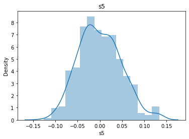
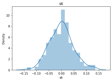
# 通过画图来查看数据分布
for col_name in dataSets.columns:
    col_data = dataSets[col_name]
    sns.distplot(col_data)
    plt.title(col_name)
    plt.show()
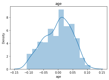
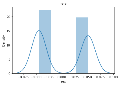
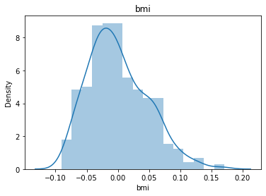
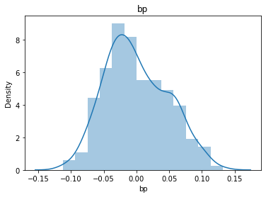
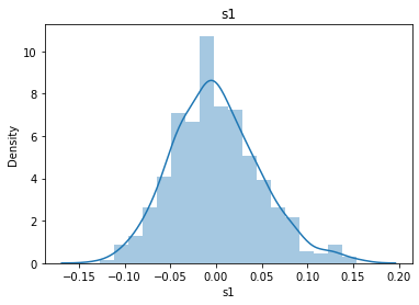
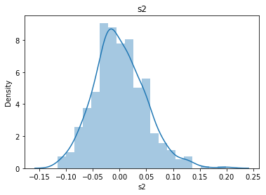
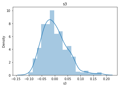
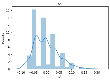
# 各种转化的目的 为了让特征值尽可能的正态分布
# 好处: 1.减少算法的迭代次数  2.数据降噪
岭回归
X W y
1 2 3 w1 1
2 3 4 w2 3
2 4 6 w3 2
a1 + b2 + c*3 =1
任何样本数据都必然拥有以下特点:
- 1. 存在噪声
- 2. 多重共线性
- 可能无法避免
如何解决这些问题呢: 角度一:算法的角度(正则项) 角度二:从数据集的角度(主要解决思路 也最有效果)
X.T *X
X W y
1+λ 2 3 w1 1
2 3+λ 4 w2 3
2 4 6+λ w3 2
y = f(x) + bias + 正则项
y = f(x) + 1 - 1
缩减算法:减少 无用特征影响系数w —>0
过拟合:模型对训练集的局部特征过度关注导致的
100收入 4身高 1地域 0.0005电话 0.01学历
岭回归的基本使用
import numpy as np
X = np.array([[1,2,3,4],[1,3,8,5]])
X
array([[1, 2, 3, 4],
       [1, 3, 8, 5]])
y = np.array([3,5])
y
array([3, 5])
from sklearn.linear_model import LinearRegression,Ridge
lr = LinearRegression()
lr.fit(X, y)
LinearRegression()
# 岭回归的使用
ridge = Ridge()
ridge.fit(X,y)
Ridge()
获取线性回归的系数
lr.coef_
array([5.55111512e-17, 7.40740741e-02, 3.70370370e-01, 7.40740741e-02])
ridge.coef_
array([0. , 0.06896552, 0.34482759, 0.06896552])
获取线性回归的截距
lr.intercept_
1.4444444444444446
ridge.intercept_
1.6206896551724141
糖尿病的回归分析
from sklearn.datasets import load_diabetes
import pandas as pd
from pandas import Series,DataFrame
import matplotlib.pyplot as plt
%matplotlib inline

from sklearn.model_selection import train_test_split
# 拿出数据
diabetes = load_diabetes()
train = diabetes.data # X
target = diabetes.target # y
feature_names = diabetes.feature_names
feature_names
['age', 'sex', 'bmi', 'bp', 's1', 's2', 's3', 's4', 's5', 's6']
# 1.实例化岭回归
ridge = Ridge(alpha=1.0)
# 2.拆分测试机和训练集
X_train, X_test, y_train, y_test = train_test_split(train,target,test_size=0.2)
# 3.模型训练
ridge.fit(X_train,y_train)
Ridge()
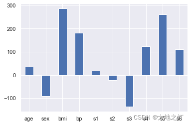
利用系数来表达各个特征对目标的影响,进而可以根据这个影响的大小来进行特征选择
ridge.coef_
array([  36.01468243,  -90.75889609,  287.47200232,  180.86788548,
         18.90897004,  -23.19316941, -137.06157738,  123.45193373,
        260.76150489,  110.61743971])
feature_names
['age', 'sex', 'bmi', 'bp', 's1', 's2', 's3', 's4', 's5', 's6']
import seaborn as sns
sns.set()
# 绘图来查看一下影响因子
importances =  Series(data=ridge.coef_,index=feature_names)
importances.plot(kind='bar')
plt.xticks(rotation=0)
plt.show()
# 在特征重要性选择中,即使负数也会影响到整体,因此我们使用绝对值进行处理
importances =  Series(data=np.abs(ridge.coef_),index=feature_names).sort_values(ascending=False)
importances.plot(kind='bar')
plt.xticks(rotation=0)
plt.show()
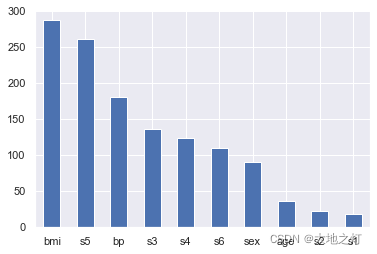
根据特征的重要性,我们发现前7个特征更加重要,因此我们可以选择前7个特征重新建模
importances
bmi    287.472002
s5     260.761505
bp     180.867885
s3     137.061577
s4     123.451934
s6     110.617440
sex     90.758896
age     36.014682
s2      23.193169
s1      18.908970
dtype: float64
importances_columns = ['bmi','s5','bp','s3','s4','s6','sex']
importances_columns
['bmi', 's5', 'bp', 's3', 's4', 's6', 'sex']
dataSets = DataFrame(data=train,columns=feature_names)
dataSets.head()
| age | sex | bmi | bp | s1 | s2 | s3 | s4 | s5 | s6 | |
|---|---|---|---|---|---|---|---|---|---|---|
| 0 | 0.038076 | 0.050680 | 0.061696 | 0.021872 | -0.044223 | -0.034821 | -0.043401 | -0.002592 | 0.019908 | -0.017646 |
| 1 | -0.001882 | -0.044642 | -0.051474 | -0.026328 | -0.008449 | -0.019163 | 0.074412 | -0.039493 | -0.068330 | -0.092204 |
| 2 | 0.085299 | 0.050680 | 0.044451 | -0.005671 | -0.045599 | -0.034194 | -0.032356 | -0.002592 | 0.002864 | -0.025930 |
| 3 | -0.089063 | -0.044642 | -0.011595 | -0.036656 | 0.012191 | 0.024991 | -0.036038 | 0.034309 | 0.022692 | -0.009362 |
| 4 | 0.005383 | -0.044642 | -0.036385 | 0.021872 | 0.003935 | 0.015596 | 0.008142 | -0.002592 | -0.031991 | -0.046641 |
X = dataSets[importances_columns]
X.head()
| bmi | s5 | bp | s3 | s4 | s6 | sex | |
|---|---|---|---|---|---|---|---|
| 0 | 0.061696 | 0.019908 | 0.021872 | -0.043401 | -0.002592 | -0.017646 | 0.050680 |
| 1 | -0.051474 | -0.068330 | -0.026328 | 0.074412 | -0.039493 | -0.092204 | -0.044642 |
| 2 | 0.044451 | 0.002864 | -0.005671 | -0.032356 | -0.002592 | -0.025930 | 0.050680 |
| 3 | -0.011595 | 0.022692 | -0.036656 | -0.036038 | 0.034309 | -0.009362 | -0.044642 |
| 4 | -0.036385 | -0.031991 | 0.021872 | 0.008142 | -0.002592 | -0.046641 | -0.044642 |
y = target
# 已经做了特征选择的数据 重新进行划分
X_train, X_test, y_train,y_test = train_test_split(X,y,test_size=0.2,random_state=1)
# 对已经使用了特征选择的数据 进行建模
ridge = Ridge(alpha=1.0)
ridge.fit(X_train,y_train)
Ridge()
from sklearn.metrics import mean_squared_error
mean_squared_error(y_test,ridge.predict(X_test))
3276.750176885635
linear = LinearRegression()
linear.fit(X_train,y_train)
LinearRegression()
mean_squared_error(y_test,linear.predict(X_test))
3080.257052972186
# 比较 没有做特征选择的样本集
X_train1,X_test1,y_train1,y_test1 = train_test_split(train,target,test_size=0.2,random_state=1)
linear = LinearRegression()
linear.fit(X_train1,y_train1)

mean_squared_error(y_test1, linear.predict(X_test1))
2992.5576814529445
# Ridge LinearRegression 的系数都可以用来做特征选择
建模的核心:
数据质量(特征工程)
其次 才是算法和调参
# 特征工程 (目的:为了让模型可以得到更好的一个数据集)
# 特征选择 (基于算法的选择 常用的算法 基于线性的 决策树的..)
# 特征提取 (基于经验提取)
# 无量纲处理 (基于标准正态分布)
# 分箱操作
# 空值填充
# 异常值过滤
lasso回归
from sklearn.linear_model import Lasso,Ridge,LinearRegression
import numpy as np
X = np.array([[1,2,3,4,5],[2,3,2,1,7]])
X
array([[1, 2, 3, 4, 5],
       [2, 3, 2, 1, 7]])
y = np.array([1,2])
y
array([1, 2])
# 使用拉索回归建模
# 1.实例化
lasso = Lasso(alpha=0.001)
# 2.训练模型
lasso.fit(X,y)
Lasso(alpha=0.001)
lasso.coef_
array([ 0. , 0. , -0. , -0.33288889, 0. ])
ridge = Ridge()
ridge.fit(X,y)
ridge.coef_
array([ 0.05555556, 0.05555556, -0.05555556, -0.16666667, 0.11111111])
linear = LinearRegression()
linear.fit(X,y)
linear.coef_
array([ 0.0625, 0.0625, -0.0625, -0.1875, 0.125 ])
三种不同的回归系数比较
a = np.array([1,2,3,4,5])
a
array([1, 2, 3, 4, 5])
a[[0,2]]= 0
a
array([0, 2, 0, 4, 5])
W[np.random.permutation(200)[10:]]
array([9.96516152e-01, 5.32391471e-01, 4.93905634e-02, 9.85577787e-01,
       8.99366918e-01, 7.54742781e-01, 3.64525327e-01, 9.63422337e-01,
       5.36894360e-01, 3.38068592e-01, 1.01662067e-01, 7.71842842e-01,
       3.54289304e-01, 4.07413512e-01, 8.47113116e-01, 5.77998640e-01,
       3.53312178e-01, 3.77569649e-02, 5.13445478e-01, 6.01971296e-01,
       2.17216303e-01, 6.06875883e-01, 1.16501776e-01, 9.29483618e-01,
       1.94729718e-01, 3.79243355e-01, 2.32664998e-01, 8.11550904e-01,
       3.45585212e-01, 8.97118361e-01, 5.18677931e-01, 4.76157464e-02,
       5.46642599e-01, 6.28107676e-01, 6.99770540e-01, 5.53885482e-01,
       1.06766013e-01, 7.41079780e-01, 9.47096359e-01, 7.76124225e-02,
       4.32180516e-01, 7.04356613e-01, 8.82416582e-01, 8.81437686e-02,
       4.85216991e-02, 4.52000028e-01, 3.82505394e-01, 9.36136345e-01,
       5.70745661e-01, 2.92274222e-01, 4.26258679e-01, 6.16950539e-01,
       5.18476200e-01, 8.96571765e-01, 3.28256203e-01, 7.68933452e-01,
       1.20772148e-01, 1.69006603e-02, 4.60183339e-01, 3.28257762e-01,
       3.98607160e-01, 8.70438678e-01, 1.51239976e-01, 7.40343824e-01,
       4.63024024e-01, 5.76156560e-01, 1.92047942e-03, 9.62859485e-01,
       7.33956356e-01, 2.39740967e-01, 1.83232929e-01, 1.00671402e-01,
       1.30679135e-01, 3.73608097e-01, 6.00838009e-01, 4.40710351e-01,
       5.70835282e-01, 2.32309233e-01, 8.87733637e-01, 6.36192443e-01,
       7.90478439e-01, 2.63124712e-01, 2.88636831e-01, 2.55830360e-02,
       4.13459126e-01, 9.72222742e-01, 6.12679019e-01, 6.05975771e-01,
       9.03416989e-01, 3.47247811e-01, 9.51756590e-01, 5.69286087e-01,
       9.65890196e-01, 5.82139890e-01, 5.51093440e-01, 5.56825893e-01,
       6.24669833e-01, 5.51314324e-01, 6.48828274e-01, 3.02442666e-01,
       6.84657374e-01, 3.71998163e-01, 7.16317195e-01, 9.65935762e-01,
       7.65903638e-01, 3.70943741e-01, 1.16563475e-01, 1.72965641e-01,
       9.18789086e-01, 8.81839640e-01, 7.13009929e-01, 6.42216668e-01,
       4.15987478e-01, 7.91627848e-02, 8.95408244e-01, 4.77017976e-01,
       8.99848891e-01, 9.69446936e-01, 9.39478644e-01, 1.77600703e-01,
       1.59593839e-01, 6.76554096e-01, 2.64041902e-01, 9.89595420e-01,
       2.90237110e-01, 4.25976169e-01, 8.44444767e-01, 2.10848895e-02,
       7.76392532e-01, 2.79007862e-01, 5.35291152e-02, 9.54334908e-01,
       8.78255077e-01, 2.58898672e-01, 3.17425087e-01, 3.63382801e-01,
       2.19014741e-01, 1.82570099e-01, 6.56801360e-01, 6.86939280e-01,
       1.08914417e-01, 1.94762611e-04, 2.22156323e-01, 3.97132753e-01,
       4.11637144e-01, 3.98905184e-01, 4.26635545e-01, 1.26789802e-01,
       4.30105437e-02, 9.35596787e-01, 3.33434333e-01, 4.57113238e-01,
       7.28383428e-01, 7.32163308e-01, 3.15656355e-02, 2.87251282e-01,
       9.53105336e-01, 6.89125739e-01, 2.34995553e-01, 9.40084446e-01,
       9.13471128e-01, 3.74629473e-01, 5.50133348e-01, 4.42872398e-01,
       6.28822215e-01, 6.61706633e-01, 6.25204117e-01, 5.80891452e-01,
       6.96894553e-01, 3.42318889e-01, 3.35023780e-01, 7.54764315e-01,
       5.51524765e-01, 7.14882962e-01, 7.97392627e-01, 8.60508187e-01,
       4.49895726e-01, 9.66104169e-01, 3.80176775e-01, 6.78332181e-01,
       6.38685181e-01, 8.87437347e-01, 5.55300557e-01, 6.84089183e-01,
       4.23983590e-01, 9.48933675e-01, 5.42585937e-01, 6.54043901e-01,
       2.96119799e-01, 2.78872800e-01])
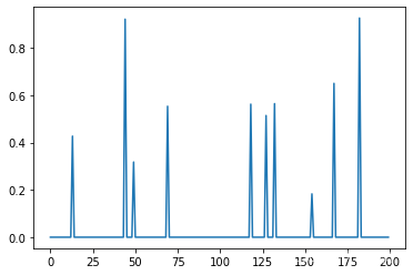
# 数据构造
samples = 50
features = 200


# 假设真实的数据中,对结果有真实作用的特征就10个
X = np.random.random(size=(samples,features))
W = np.random.random(features)

# W 这两百个数据中(系数),只有随机的10个是非0 其他都是0
W[np.random.permutation(200)[10:]] = 0

y = np.dot(X,W)
W
array([0.        , 0.        , 0.        , 0.        , 0.        ,
       0.        , 0.        , 0.        , 0.        , 0.        ,
       0.        , 0.        , 0.        , 0.4271518 , 0.        ,
       0.        , 0.        , 0.        , 0.        , 0.        ,
       0.        , 0.        , 0.        , 0.        , 0.        ,
       0.        , 0.        , 0.        , 0.        , 0.        ,
       0.        , 0.        , 0.        , 0.        , 0.        ,
       0.        , 0.        , 0.        , 0.        , 0.        ,
       0.        , 0.        , 0.        , 0.        , 0.92177717,
       0.        , 0.        , 0.        , 0.        , 0.31777111,
       0.        , 0.        , 0.        , 0.        , 0.        ,
       0.        , 0.        , 0.        , 0.        , 0.        ,
       0.        , 0.        , 0.        , 0.        , 0.        ,
       0.        , 0.        , 0.        , 0.        , 0.55356324,
       0.        , 0.        , 0.        , 0.        , 0.        ,
       0.        , 0.        , 0.        , 0.        , 0.        ,
       0.        , 0.        , 0.        , 0.        , 0.        ,
       0.        , 0.        , 0.        , 0.        , 0.        ,
       0.        , 0.        , 0.        , 0.        , 0.        ,
       0.        , 0.        , 0.        , 0.        , 0.        ,
       0.        , 0.        , 0.        , 0.        , 0.        ,
       0.        , 0.        , 0.        , 0.        , 0.        ,
       0.        , 0.        , 0.        , 0.        , 0.        ,
       0.        , 0.        , 0.        , 0.56237781, 0.        ,
       0.        , 0.        , 0.        , 0.        , 0.        ,
       0.        , 0.        , 0.51434962, 0.        , 0.        ,
       0.        , 0.        , 0.56461673, 0.        , 0.        ,
       0.        , 0.        , 0.        , 0.        , 0.        ,
       0.        , 0.        , 0.        , 0.        , 0.        ,
       0.        , 0.        , 0.        , 0.        , 0.        ,
       0.        , 0.        , 0.        , 0.        , 0.18319368,
       0.        , 0.        , 0.        , 0.        , 0.        ,
       0.        , 0.        , 0.        , 0.        , 0.        ,
       0.        , 0.        , 0.65038963, 0.        , 0.        ,
       0.        , 0.        , 0.        , 0.        , 0.        ,
       0.        , 0.        , 0.        , 0.        , 0.        ,
       0.        , 0.        , 0.92661222, 0.        , 0.        ,
       0.        , 0.        , 0.        , 0.        , 0.        ,
       0.        , 0.        , 0.        , 0.        , 0.        ,
       0.        , 0.        , 0.        , 0.        , 0.        ])
import matplotlib.pyplot as plt
%matplotlib inline
plt.plot(W)
[<matplotlib.lines.Line2D at 0x1c8ea5fcf40>]
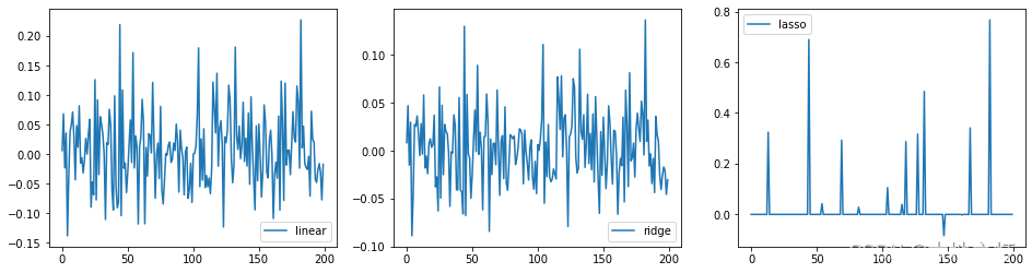
# 针对实战情况,三种不同的回归对比
# 1.实例化
linear = LinearRegression()
ridge = Ridge(alpha=10)
lasso = Lasso(alpha=0.01)

# 2.训练
linear.fit(X,y)
ridge.fit(X,y)
lasso.fit(X,y)

# 画图
plt.figure(figsize=(16,4))

ax1 = plt.subplot(1, 3, 1)
plt.plot(linear.coef_,label='linear')
plt.legend()

ax2 = plt.subplot(1,3,2)
plt.plot(ridge.coef_,label ='ridge')
plt.legend()

ax3 = plt.subplot(1,3,3)
plt.plot(lasso.coef_,label='lasso')
plt.legend()
<matplotlib.legend.Legend at 0x1c8ea6b7b50>