《机器学习》------实验五（综合实验）

实验内容：

使用CTG数据将胎儿的健康分为正常，可疑或病理性。

数据描述：

对胎儿健康进行分类，以防止儿童和产妇死亡。
降低儿童死亡率反映在联合国的若干可持续发展目标中，是人类进步的关键指标。联合国预计，到2030年，各国将结束可预防的5岁以下新生儿和儿童的死亡，所有国家都力争将5岁以下儿童的死亡率降低到至少每1000活产25人。
与儿童死亡率的概念平行的当然是孕产妇死亡率，其占妊娠和分娩期间和之后（截至2017年）的295 000例死亡。这些死亡中的绝大多数（94％）发生在资源贫乏的地区，大多数可以预防。
鉴于上述情况，心电图（CTG）是评估胎儿健康的一种简单且成本可承受的选择，允许医疗保健专业人员采取行动以预防儿童和孕产妇死亡。该设备本身通过发送超声波脉冲并读取其响应来工作，从而减轻了胎儿心率（FHR），胎儿运动，子宫收缩等方面的负担。

内容范围：

该数据集包含从心电图检查中提取的2126条特征记录，然后由三名产科专家将其分类为3类：

1. 正常
2. 疑似
3. 病理性的

创建一个多类模型以将CTG功能分类为三种胎儿健康状态。
“train.csv”包含1767个数据，每个数据包含21个属性。最后一列“fetal_health”的值表示健康程度，为分类标签，其中“1”为正常，“2”为疑似，“3”为病例性的。
“test.csv”包含280个数据，你的目标是预测其结果。
“predict.csv”是需要将预测的结果放在此表中，然后上传。

要求：

1. 在数据理解和清洗中，要求将按属性进行数据分析，统计信息缺失情况，且以图表的形式对数据进行展示。
2. 在特征提取和选择中，要求对清洗后的数据进行特征提取，选择合适的特征或使用降维作为模型训练的输入。
3. 在模型构建中，要求选择合适的机器学习方法构建模型（可选择多种方法进行对比），输出在训练集上的准确率，要有训练过程。在此部分，要对使用的方法进行方法介绍。（以SVM为例，要阐述SVM的基本原理、算法流程、目标函数等）。
4. 在模型评估和预测中，要求使用预测数据集预测结果，将预测结果保存到predict.csv文件中。与真实标签对比，输出测试集上的准确率。

实验报告（文档）内应将过程分为以下几步：
1.数据理解和清洗；
2.特征提取和选择；
3.构建模型进行训练；
4.模型评估和预测。

数据处理的具体过程可参考泰坦尼克号的例子：https://zhuanlan.zhihu.com/p/342552186

数据集：https://pan.baidu.com/s/1VZTWItjp2XiztUjGtO7Tqw
提取码：5613

1.数据理解和清洗：

# 1、数据理解和清洗：
train_path = "F:/研究生/课程/机器学习/综合实验/train.csv"
test_path = "F:/研究生/课程/机器学习/综合实验/test.xlsx"
Data_train = pd.read_csv(train_path)
Data_test = pd.read_excel(test_path)
# 查看属性的数据量和缺失值情况：
print(Data_train.info())
print(Data_test.info())

# 查看各属性的基本信息：
pd.set_option('display.max_columns',None)
print(Data_train.describe())
print(Data_test.describe())

# 查看分类情况：
# 显示中文标题
plt.rcParams['font.sans-serif'] = ['SimHei']
plt.rcParams['axes.unicode_minus'] = False
print(Data_train['fetal_health'].value_counts())

首先是数据的基本统计分析：
查看数据量以及缺失值情况

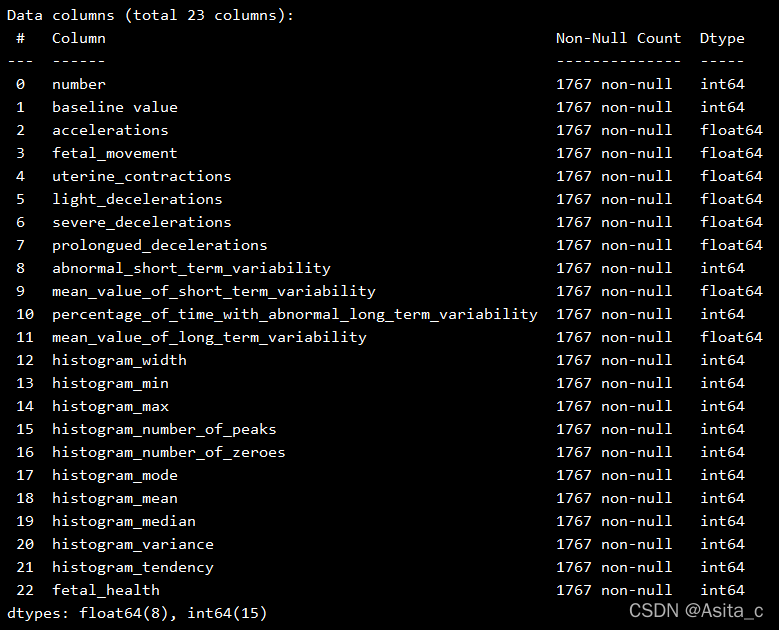
数据的属性探测：
部分属性截图：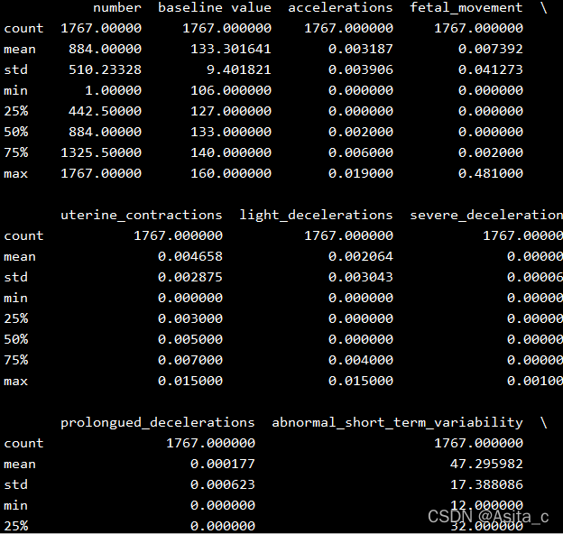
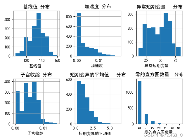
分别看一下各属性的基本分布情况，首先我们对适合利用图形展示的属性，通过绘图的方式探查部分属性的分布：

# 查看分类情况：
# 显示中文标题
plt.rcParams['font.sans-serif'] = ['SimHei']
plt.rcParams['axes.unicode_minus'] = False
print(Data_train['fetal_health'].value_counts())
 # 绘图
fig = plt.figure()
# 基线值分布
plt.subplot2grid((2, 3), (0, 0))
Data_train['baseline value'].hist()
plt.xlabel(u'基线值 ')
plt.title(u'基线值 分布')
# 加速度分布
plt.subplot2grid((2, 3), (0, 1))
Data_train['accelerations'].hist()
plt.xlabel(u'加速度 ')
plt.title(u'加速度 分布')
# 异常短期变量
plt.subplot2grid((2, 3), (0, 2))
Data_train['abnormal_short_term_variability'].hist()
plt.xlabel(u'异常短期变量   ')
plt.title(u'异常短期变量   分布')
# 子宫收缩
plt.subplot2grid((2, 3), (1, 0))
Data_train['uterine_contractions'].hist()
plt.xlabel(u'子宫收缩 ')
plt.title(u'子宫收缩 分布')
# 短期变异的平均值
plt.subplot2grid((2, 3), (1, 1))
Data_train['mean_value_of_short_term_variability'].hist()
plt.xlabel(u'短期变异的平均值   ')
plt.title(u'短期变异的平均值   分布')
# 延长 减速
plt.subplot2grid((2, 3), (1, 2))
Data_train['histogram_number_of_zeroes'].value_counts().plot(kind='bar')
plt.xlabel(u'零的直方图数量 ')
plt.title(u'零的直方图数量  分布')
plt.show()

2.特征提取和选择：

采用PCA降维，个人理解的是特征选择后的特征相当于是剔除掉一些关联性较低的，类似于一种对特征进行阉割的手法，而降维则是相当于是一种对特征空间进行压缩。

# 特征提取(降维)：
# 训练集：
y_train = np.array(Data_train)
y_train = np.mat(y_train)
y_train1 = y_train[:1000,22]
y_test1 = y_train[1000:,22]
y_train1 = np.array(y_train1)
# print(y_train)
x_train = np.array(Data_train)
x_train1 = np.mat(x_train)
x_train1 = x_train[:1000,1:22]
x_test1 =  x_train[1000:,1:22]
pca = PCA(n_components=2)
reduced_x = pca.fit_transform(x_train1)#得到了pca降到2维的数据
# print(reduced_x)
# 测试集：
x_test = np.array(Data_test)
x_test = np.mat(x_test)
x_test = x_test[:,1:22]
pca = PCA(n_components=2)
reduced_test = pca.fit_transform(x_test)#得到了pca降到2维的数据

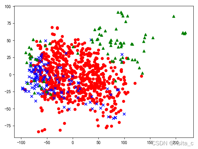
显示降维后的数据集：

# 训练集降维后的散点图
red_x, red_y = [], []
blue_x, blue_y = [], []
grenn_x, green_y = [], []
for i in range(len(reduced_x)):
    if y_train1[i] ==1:
        red_x.append(reduced_x[i][0])
        red_y.append(reduced_x[i][1])
    elif y_train1[i] ==2:
        blue_x.append(reduced_x[i][0])
        blue_y.append(reduced_x[i][1])
    elif y_train1[i] ==3:
        grenn_x.append(reduced_x[i][0])
        green_y.append(reduced_x[i][1])
plt.scatter(red_x, red_y, c='r', marker='o')
plt.scatter(blue_x, blue_y, c='b', marker='x')
plt.scatter(grenn_x, green_y, c='g', marker='^')
plt.show()

3.构建模型进行训练：

选取了两种算法进行训练，
第一种是SVM：
因为只给了训练集，并且测试集没有标签，是需要把结果输出作为测试集的标签来发给老师计算模型准确率的，因此，这里把训练集再次划分为训练集和测试集：

# 训练集：
y_train = np.array(Data_train)
y_train = np.mat(y_train)
y_train1 = y_train[:1000,22]
y_test1 = y_train[1000:,22]
y_train1 = np.array(y_train1)
print(y_train)
x_train = np.array(Data_train)
x_train1 = np.mat(x_train)
x_train1 = x_train[:1000,1:22]
x_test1 =  x_train[1000:,1:22]
# 测试集：
x_test = np.array(Data_test)
x_test = np.mat(x_test)
x_test = x_test[:,1:22]

SVM分类器参数配置、训练：

# SVM分类器参数设置
clf = svm.SVC(C=1,  # 误差项惩罚系数,默认值是1
                  kernel='linear',  # 线性核
                  decision_function_shape='ovr')  # 决策函数

# 模型训练
def train(clf, x_train, y_train):
    clf.fit(x_train,  # 训练集特征向量
            y_train.ravel())  # 训练集目标值

# 训练SVM模型
train(clf, x_train1, y_train1)

第二种是使用的集成学习方法，Adaboost算法进行学习

# 单棵决策树
clf = DecisionTreeClassifier(max_depth=3)
clf.fit(x_train1,y_train1)
# Adaboost
clf = AdaBoostClassifier(DecisionTreeClassifier(max_depth=3,min_samples_split=2),
                         n_estimators=50,algorithm="SAMME",learning_rate=0.8)
clf.fit(x_train1,y_train1)

4.模型评估和预测（对比算法）：

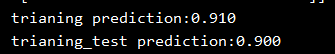
SVM：

# 输出准确率
# 训练集：
print('trianing prediction:%.3f' %(clf.score(x_train1, y_train1)))
print('trianing_test prediction:%.3f' %(clf.score(x_test1, y_test1)))
test_predict = clf.predict(x_test)
print(test_predict)
print((clf.predict(x_test)==1).sum())
print((clf.predict(x_test)==2).sum())
print((clf.predict(x_test)==3).sum())

Adaboost：

# 输出准确率
print('训练集正确率：',accuracy_score(y_train1,clf.predict(x_train1)))
print('测试集正确率：',accuracy_score(y_test1,clf.predict(x_test1)))
test_predict = clf.predict(x_test)
print("1",(test_predict==1).sum())
print("2",(test_predict==2).sum())
print("3",(test_predict==3).sum())

可以看到，Adaboost将迭代次数设置为50次时，弱分类器选择的是单颗决策树，通过集成学习的方法得到的模型准确率明显优于传统的SVM方法。

5.将预测结果输出到 practice.csv

# 将预测结果写入到指定excel中
workbook = xlwt.Workbook(encoding='utf-8')
bg = op.load_workbook(r"F:/研究生/课程/机器学习/综合实验/predict.xlsx")
sheet = bg["Sheet1"]
for i in range(len(test_predict)):
    sheet.cell(i+2,2,test_predict[i])
bg.save(r"F:/研究生/课程/机器学习/综合实验/predict.xlsx")

SVM方式完整代码：

#作   者：Asita
#开发时间：2021/12/3 19:24
import numpy as np
import pandas as pd
import matplotlib.pyplot as plt
from sklearn import svm
from sklearn.decomposition import PCA
import xlwt
import openpyxl as op
# 1、数据理解和清洗：
train_path = "F:/研究生/课程/机器学习/综合实验/train.csv"
test_path = "F:/研究生/课程/机器学习/综合实验/test.xlsx"
Data_train = pd.read_csv(train_path)
Data_test = pd.read_excel(test_path)

# 查看属性的数据量和缺失值情况：
print(Data_train.info())
print(Data_test.info())

# 查看各属性的基本信息：
pd.set_option('display.max_columns',None)
print(Data_train.describe())
print(Data_test.describe())

# 查看分类情况：
# 显示中文标题
plt.rcParams['font.sans-serif'] = ['SimHei']
plt.rcParams['axes.unicode_minus'] = False
print(Data_train['fetal_health'].value_counts())
 # 绘图
fig = plt.figure()
# 基线值分布
plt.subplot2grid((2, 3), (0, 0))
Data_train['baseline value'].hist()
plt.xlabel(u'基线值 ')
plt.title(u'基线值 分布')
# 加速度分布
plt.subplot2grid((2, 3), (0, 1))
Data_train['accelerations'].hist()
plt.xlabel(u'加速度 ')
plt.title(u'加速度 分布')
# 异常短期变量
plt.subplot2grid((2, 3), (0, 2))
Data_train['abnormal_short_term_variability'].hist()
plt.xlabel(u'异常短期变量   ')
plt.title(u'异常短期变量   分布')
# 子宫收缩
plt.subplot2grid((2, 3), (1, 0))
Data_train['uterine_contractions'].hist()
plt.xlabel(u'子宫收缩 ')
plt.title(u'子宫收缩 分布')
# 短期变异的平均值
plt.subplot2grid((2, 3), (1, 1))
Data_train['mean_value_of_short_term_variability'].hist()
plt.xlabel(u'短期变异的平均值   ')
plt.title(u'短期变异的平均值   分布')
# 延长 减速
plt.subplot2grid((2, 3), (1, 2))
Data_train['histogram_number_of_zeroes'].value_counts().plot(kind='bar')
plt.xlabel(u'零的直方图数量 ')
plt.title(u'零的直方图数量  分布')
plt.show()

# 特征提取(降维)：
# 训练集：
y_train = np.array(Data_train)
y_train = np.mat(y_train)
y_train1 = y_train[:1000,22]
y_test1 = y_train[1000:,22]
y_train1 = np.array(y_train1)
print(y_train)
x_train = np.array(Data_train)
x_train1 = np.mat(x_train)
x_train1 = x_train[:1000,1:22]
x_test1 =  x_train[1000:,1:22]
pca = PCA(n_components=2)
reduced_x = pca.fit_transform(x_train1)#得到了pca降到2维的数据
print(reduced_x)
# 测试集：
x_test = np.array(Data_test)
x_test = np.mat(x_test)
x_test = x_test[:,1:22]
pca = PCA(n_components=2)
reduced_test = pca.fit_transform(x_test)#得到了pca降到2维的数据
print(reduced_test)
# 训练集降维后的散点图
red_x, red_y = [], []
blue_x, blue_y = [], []
grenn_x, green_y = [], []
for i in range(len(reduced_x)):
    if y_train1[i] ==1:
        red_x.append(reduced_x[i][0])
        red_y.append(reduced_x[i][1])
    elif y_train1[i] ==2:
        blue_x.append(reduced_x[i][0])
        blue_y.append(reduced_x[i][1])
    elif y_train1[i] ==3:
        grenn_x.append(reduced_x[i][0])
        green_y.append(reduced_x[i][1])
plt.scatter(red_x, red_y, c='r', marker='o')
plt.scatter(blue_x, blue_y, c='b', marker='x')
plt.scatter(grenn_x, green_y, c='g', marker='^')
plt.show()

# SVM分类器参数设置
clf = svm.SVC(C=1,  # 误差项惩罚系数,默认值是1
                  kernel='linear',  # 线性核
                  decision_function_shape='ovr')  # 决策函数

# 模型训练
def train(clf, x_train, y_train):
    clf.fit(x_train,  # 训练集特征向量
            y_train.ravel())  # 训练集目标值

# 训练SVM模型
train(clf, x_train1, y_train1)

# 输出准确率
# 训练集：
print('trianing prediction:%.3f' %(clf.score(x_train1, y_train1)))
print('trianing_test prediction:%.3f' %(clf.score(x_test1, y_test1)))
test_predict = clf.predict(x_test)
print(test_predict)
print((clf.predict(x_test)==1).sum())
print((clf.predict(x_test)==2).sum())
print((clf.predict(x_test)==3).sum())

# 将预测结果写入到指定excel中
workbook = xlwt.Workbook(encoding='utf-8')
bg = op.load_workbook(r"F:/研究生/课程/机器学习/综合实验/predict.xlsx")
sheet = bg["Sheet1"]
for i in range(len(test_predict)):
    sheet.cell(i+2,2,test_predict[i])
bg.save(r"F:/研究生/课程/机器学习/综合实验/predict.xlsx")

Adaboost方式完整代码：

#作   者：Asita
#开发时间：2021/12/11 22:36
import numpy as np
import pandas as pd
import matplotlib.pyplot as plt
from sklearn.decomposition import PCA
import xlwt
from sklearn.tree import DecisionTreeClassifier
import openpyxl as op
from sklearn.metrics import accuracy_score
from sklearn.ensemble import AdaBoostClassifier


#去忽略warnings警告
import warnings
warnings.filterwarnings("ignore")
# 1、数据理解和清洗：
train_path = "F:/研究生/课程/机器学习/综合实验/train.csv"
test_path = "F:/研究生/课程/机器学习/综合实验/test.xlsx"
Data_train = pd.read_csv(train_path)
Data_test = pd.read_excel(test_path)
# 查看属性的数据量和缺失值情况：
print(Data_train.info())
print(Data_test.info())

# 查看各属性的基本信息：
pd.set_option('display.max_columns',None)
print(Data_train.describe())
print(Data_test.describe())

# 查看分类情况：
# 显示中文标题
plt.rcParams['font.sans-serif'] = ['SimHei']
plt.rcParams['axes.unicode_minus'] = False
print(Data_train['fetal_health'].value_counts())
 # 绘图
fig = plt.figure()
# 基线值分布
plt.subplot2grid((2, 3), (0, 0))
Data_train['baseline value'].hist()
plt.xlabel(u'基线值 ')
plt.title(u'基线值 分布')
# 加速度分布
plt.subplot2grid((2, 3), (0, 1))
Data_train['accelerations'].hist()
plt.xlabel(u'加速度 ')
plt.title(u'加速度 分布')
# 异常短期变量
plt.subplot2grid((2, 3), (0, 2))
Data_train['abnormal_short_term_variability'].hist()
plt.xlabel(u'异常短期变量   ')
plt.title(u'异常短期变量   分布')
# 子宫收缩
plt.subplot2grid((2, 3), (1, 0))
Data_train['uterine_contractions'].hist()
plt.xlabel(u'子宫收缩 ')
plt.title(u'子宫收缩 分布')
# 短期变异的平均值
plt.subplot2grid((2, 3), (1, 1))
Data_train['mean_value_of_short_term_variability'].hist()
plt.xlabel(u'短期变异的平均值   ')
plt.title(u'短期变异的平均值   分布')
# 延长 减速
plt.subplot2grid((2, 3), (1, 2))
Data_train['histogram_number_of_zeroes'].value_counts().plot(kind='bar')
plt.xlabel(u'零的直方图数量 ')
plt.title(u'零的直方图数量  分布')
plt.show()

# 特征提取(降维)：
# 训练集：
y_train = np.array(Data_train)
y_train = np.mat(y_train)
y_train1 = y_train[:1000,22]
y_test1 = y_train[1000:,22]
y_train1 = np.array(y_train1)
# print(y_train)
x_train = np.array(Data_train)
x_train1 = np.mat(x_train)
x_train1 = x_train[:1000,1:22]
x_test1 =  x_train[1000:,1:22]
pca = PCA(n_components=2)
reduced_x = pca.fit_transform(x_train1)#得到了pca降到2维的数据
# print(reduced_x)
# 测试集：
x_test = np.array(Data_test)
x_test = np.mat(x_test)
x_test = x_test[:,1:22]
pca = PCA(n_components=2)
reduced_test = pca.fit_transform(x_test)#得到了pca降到2维的数据
# print(reduced_test)
# 训练集降维后的散点图
red_x, red_y = [], []
blue_x, blue_y = [], []
grenn_x, green_y = [], []
for i in range(len(reduced_x)):
    if y_train1[i] ==1:
        red_x.append(reduced_x[i][0])
        red_y.append(reduced_x[i][1])
    elif y_train1[i] ==2:
        blue_x.append(reduced_x[i][0])
        blue_y.append(reduced_x[i][1])
    elif y_train1[i] ==3:
        grenn_x.append(reduced_x[i][0])
        green_y.append(reduced_x[i][1])
plt.scatter(red_x, red_y, c='r', marker='o')
plt.scatter(blue_x, blue_y, c='b', marker='x')
plt.scatter(grenn_x, green_y, c='g', marker='^')
plt.show()

# 单棵决策树
clf = DecisionTreeClassifier(max_depth=3)
clf.fit(x_train1,y_train1)
# Adaboost
clf = AdaBoostClassifier(DecisionTreeClassifier(max_depth=3,min_samples_split=2),
                         n_estimators=50,algorithm="SAMME",learning_rate=0.8)
clf.fit(x_train1,y_train1)

# 输出准确率
print('训练集正确率：',accuracy_score(y_train1,clf.predict(x_train1)))
print('测试集正确率：',accuracy_score(y_test1,clf.predict(x_test1)))
test_predict = clf.predict(x_test)
print("1",(test_predict==1).sum())
print("2",(test_predict==2).sum())
print("3",(test_predict==3).sum())

# 将预测结果写入到指定excel中
workbook = xlwt.Workbook(encoding='utf-8')
bg = op.load_workbook(r"F:/研究生/课程/机器学习/综合实验/predict.xlsx")
sheet = bg["Sheet1"]
for i in range(len(test_predict)):
    sheet.cell(i+2,2,test_predict[i])
bg.save(r"F:/研究生/课程/机器学习/综合实验/predict.xlsx")