机器翻译Machine Translation及其Tensorflow代码实现（含注意力attention）

机器翻译

翻译句子$x$从一种语言（源语言）到句子$y$另一种语言（目标语言）。下面这个例子就是从法语转换成为英文。

统计机器翻译

英文是Statistical Machine Translation (SMT)。核心思想是从数据中学习概率模型。
$$\begin{gathered} argma{x}_{y}P(y|x) \\ =argma{x}_{y}P(x|y)P(y) \end{gathered}$$
公式前一部分$P(x|y)$是翻译模型，负责翻译词和词组。后一部分$P(y)$是语言模型，负责使译文更加流畅。

优点

1. 思路容易理解，有可解释性

缺点

1. 需要大量的特征工程，耗费人力
2. 空间复杂度较高，需要存储额外资源，例如平行语句

对齐

为了训练出一个性能优秀的翻译模型，我们首先需要有很多的平行数据（从原文到译文）。这就需要引出对齐的概念。找到原文中的哪个短语对应到译文中的哪个短语。我们用$a$代表对齐。因此，我们的翻译模型从最大化$P(x|y)$变成了最大化$P(x,a|y)$。对齐的难点就在于原文中可能存在词语没有对应的译文(counterpart)。我们还需要考虑单词在句子中不同位置导致对句意产生的不同的影响。

即便能够进行对应，对齐本身也十分复杂，有可能出现以下3种情况。

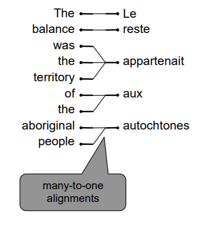
多对一

多个译文词组对应一个原文词组。

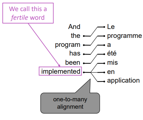
一对多

一个译文词组对应多个原文词组。类似的词被称为多产词(fertile word)。

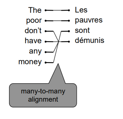
多对多

多个译文词组对应多个原文词组。无法进行更细致的拆分。

解码

在对齐之后，我们需要进行翻译。如果使用暴力方法，即枚举所有可能的译文并计算其概率，显然不太现实，因为复杂度太高。更有效的方法是进行启发式搜索算法(heuristic search algorithm)，放弃探索所有可能性较小的译文。

神经机器翻译

英文是Neural Machine Translation (NMT)。模型架构是序列到序列模型(sequence-to-sequence, seq2seq)，详情请参见我的另一篇博客。

在NMT中，我们直接计算$P(y|x)$而不是像SMT拆开计算。
$$P(y|x)=P(y_1|x)P(y_2|y_1,x)...P(y_T|y_1,...,y_{T-1},x)$$
不过，在训练过程中，我们仍然需要大量的平行语料。

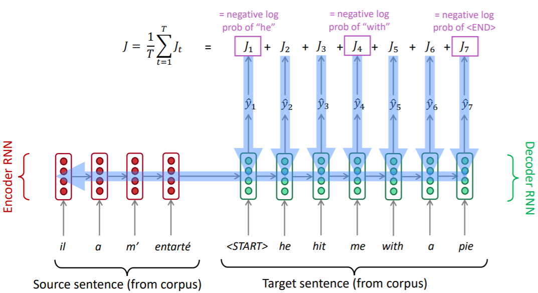
在$argmaxP(y|x)$的过程中，我们可以进行贪心搜索或者束搜索(Beam search)，虽然不保证能找到最佳的解决方案，但是大概率会找到一个还不错的译文。如果使用贪心搜索，解码会在<End>词出现后停止。但如果使用束搜索，那么不同假设会在不同时间步输出<End>词，所以我们可以预先设置一个时间步界限（到达时间$t$之后停止）或者完整译文个数的界限（输出了$n$个完整译文之后停止）作为搜索的停止条件。

另外，我们需要对损失函数进行归一化，否则模型会倾向于输出短句。
$$J=\frac{1}{t}\sum _{i=1}^{t}log{P}_{LM}(y_i|y_1,...,y_{i-1},x)$$
优点

1. 充分利用上下文，译文更流畅
2. 只需要对端到端模型的优化，不需要对子系统单独进行优化
3. 无需特征工程，减少人工

缺点

1. 解释性较差
2. 难以人工规定翻译输出规则（例如规定某个特定词组的翻译、去除偏见等）

评测

最常见的就是Bilingual Evaluation Understudy (BLEU)。

BLEU将机器翻译的译文与数个人工翻译进行比较并计算相似度。得分基于：(1) n-gram准确率（1~4-grams）；(2) 对超短句的惩罚。

该评测标准很有用，但并不完美。好的翻译有可能因为其与评测使用的翻译的n-gram重叠度较低而得到较差的BLEU分数。

代码实现

使用Tensorflow 2为框架构建。强烈建议未接触seq2seq模型的读者先读相关博客(上文给出了链接)。

准备工作

引入需要的包。下载需要的数据（http://www.manythings.org/anki/上的一个数据集）。目标是将西班牙语翻译为英语。

import re
import os
import io
import time
import unicodedata
import numpy as np
import matplotlib.pyplot as plt
import matplotlib.ticker as ticker

from sklearn.model_selection import train_test_split
import tensorflow as tf

# Download the file
path_to_zip = tf.keras.utils.get_file(
    'spa-eng.zip', origin='http://storage.googleapis.com/download.tensorflow.org/data/spa-eng.zip',
    extract=True)

path_to_file = os.path.dirname(path_to_zip)+"/spa-eng/spa.txt"

数据预处理

先定义一些特殊符号。其中“<pad>”（padding）符号用来添加在较短序列后，直到每个序列等长，而“<bos>”和“<eos>”符号分别表示序列的开始和结束。

BOS, EOS = '<bos>', '<eos>'

# Converts the unicode file to ascii
def unicode_to_ascii(s):
  return ''.join(c for c in unicodedata.normalize('NFD', s) if unicodedata.category(c) != 'Mn')

def preprocess_sentence(w):
  w = unicode_to_ascii(w.lower().strip())
  # 在单词与跟在其后的标点符号之间插入一个空格
  w = re.sub(r"([?.!,¿])", r" \1 ", w)
  w = re.sub(r'[" "]+', " ", w)
  # replacing everything with space except (a-z, A-Z, ".", "?", "!", ",")
  w = re.sub(r"[^a-zA-Z?.!,¿]+", " ", w)
  w = w.strip()
  w = BOS + ' ' + w + ' ' + EOS
  return w

# 去除重音符号，返回单词对：[ENGLISH, SPANISH]
def create_dataset(path, num_examples):
  lines = io.open(path, encoding='UTF-8').read().strip().split('\n')
  word_pairs = [[preprocess_sentence(w) for w in l.split('\t')] for l in lines[:num_examples]]
  return zip(*word_pairs)

# 将一个序列中所有的词记录在all_tokens中以便之后构造词典，然后在该序列后面添加PAD直到序列
def tokenize(lang):
  ## reserve all punctuations
  lang_tokenizer = tf.keras.preprocessing.text.Tokenizer(filters='')
  lang_tokenizer.fit_on_texts(lang)
  tensor = lang_tokenizer.texts_to_sequences(lang)
  tensor = tf.keras.preprocessing.sequence.pad_sequences(tensor, padding='post')
  return tensor, lang_tokenizer

def load_dataset(path, num_examples=None):
  targ_lang, inp_lang = create_dataset(path, num_examples)
  input_tensor, inp_lang_tokenizer = tokenize(inp_lang)
  target_tensor, targ_lang_tokenizer = tokenize(targ_lang)
  return input_tensor, target_tensor, inp_lang_tokenizer, targ_lang_tokenizer

# display index to word mapping
def convert(lang, tensor):
  for t in tensor:
    if t!=0:
      print ("%d ----> %s" % (t, lang.index_word[t]))

num_examples = 1000 ##可供调整
input_tensor, target_tensor, inp_lang, targ_lang = load_dataset(path_to_file, num_examples)
max_length_targ, max_length_inp = target_tensor.shape[1], input_tensor.shape[1]
input_tensor_train, input_tensor_val, target_tensor_train, target_tensor_val = train_test_split(input_tensor, target_tensor, test_size=0.2)
print(len(input_tensor_train), len(target_tensor_train), len(input_tensor_val), len(target_tensor_val))

下面设置一些模型训练时候的超参数。

BUFFER_SIZE = len(input_tensor_train)
BATCH_SIZE = 32
steps_per_epoch = len(input_tensor_train)//BATCH_SIZE
embedding_dim = 256
units = 1024
vocab_inp_size = len(inp_lang.word_index)+1
vocab_tar_size = len(targ_lang.word_index)+1

dataset = tf.data.Dataset.from_tensor_slices((input_tensor_train, target_tensor_train)).shuffle(BUFFER_SIZE)
dataset = dataset.batch(BATCH_SIZE, drop_remainder=True)
example_input_batch, example_target_batch = next(iter(dataset))
example_input_batch.shape, example_target_batch.shape

编码器、解码器和注意力机制

我们先创建编码器。

class Encoder(tf.keras.Model):
  def __init__(self, vocab_size, embedding_dim, enc_units, batch_sz):
    super(Encoder, self).__init__()
    self.batch_sz = batch_sz
    self.enc_units = enc_units
    self.embedding = tf.keras.layers.Embedding(vocab_size, embedding_dim)
    self.gru = tf.keras.layers.GRU(self.enc_units, return_sequences=True,
          return_state=True, recurrent_initializer='glorot_uniform')

  def call(self, x, hidden):
    x = self.embedding(x)
    output, state = self.gru(x, initial_state=hidden)
    return output, state

  def initialize_hidden_state(self):
    return tf.zeros((self.batch_sz, self.enc_units))

encoder = Encoder(vocab_inp_size, embedding_dim, units, BATCH_SIZE)
sample_hidden = encoder.initialize_hidden_state()
sample_output, sample_hidden = encoder(example_input_batch, sample_hidden)
print ('Encoder output shape: (batch size, sequence length, units) {}'.format(sample_output.shape))
print ('Encoder Hidden state shape: (batch size, units) {}'.format(sample_hidden.shape))

然后实现注意力机制。此处采用的是加法注意力。

class BahdanauAttention(tf.keras.layers.Layer):
  def __init__(self, units):
    super(BahdanauAttention, self).__init__()
    self.W1 = tf.keras.layers.Dense(units)
    self.W2 = tf.keras.layers.Dense(units)
    self.V = tf.keras.layers.Dense(1)

  def call(self, query, values):
    # query hidden state shape == (batch_size, hidden size)
    # query_with_time_axis shape == (batch_size, 1, hidden size)
    # values shape == (batch_size, max_len, hidden size)
    # we are doing this to broadcast addition along the time axis to calculate the score
    query_with_time_axis = tf.expand_dims(query, 1)

    # score shape == (batch_size, max_length, 1)
    # we get 1 at the last axis because we are applying score to self.V
    # the shape of the tensor before applying self.V is (batch_size, max_length, units)
    score = self.V(tf.nn.tanh(self.W1(query_with_time_axis) + self.W2(values)))

    # attention_weights shape == (batch_size, max_length, 1)
    attention_weights = tf.nn.softmax(score, axis=1)

    # context_vector shape after sum == (batch_size, hidden_size)
    context_vector = attention_weights * values
    context_vector = tf.reduce_sum(context_vector, axis=1)

    return context_vector, attention_weights

attention_layer = BahdanauAttention(10)
attention_result, attention_weights = attention_layer(sample_hidden, sample_output)
print("Attention result shape: (batch size, units) {}".format(attention_result.shape))
print("Attention weights shape: (batch_size, sequence_length, 1) {}".format(attention_weights.shape))

最后，实现解码器。

class Decoder(tf.keras.Model):
  def __init__(self, vocab_size, embedding_dim, dec_units, batch_sz):
    super(Decoder, self).__init__()
    self.batch_sz = batch_sz
    self.dec_units = dec_units
    self.embedding = tf.keras.layers.Embedding(vocab_size, embedding_dim)
    self.gru = tf.keras.layers.GRU(self.dec_units, return_sequences=True,
          return_state=True, recurrent_initializer='glorot_uniform')
    self.fc = tf.keras.layers.Dense(vocab_size)

    # used for attention
    self.attention = BahdanauAttention(self.dec_units)

  def call(self, x, hidden, enc_output):
    # enc_output shape == (batch_size, max_length, hidden_size)
    context_vector, attention_weights = self.attention(hidden, enc_output)
    # x shape after passing through embedding == (batch_size, 1, embedding_dim)
    x = self.embedding(x)
    # x shape after concatenation == (batch_size, 1, embedding_dim + hidden_size)
    x = tf.concat([tf.expand_dims(context_vector, 1), x], axis=-1)
    # passing the concatenated vector to the GRU
    output, state = self.gru(x)
    # output shape == (batch_size * 1, hidden_size)
    output = tf.reshape(output, (-1, output.shape[2]))
    # output shape == (batch_size, vocab)
    x = self.fc(output)
    return x, state, attention_weights

decoder = Decoder(vocab_tar_size, embedding_dim, units, BATCH_SIZE)
sample_decoder_output, _, _ = decoder(tf.random.uniform((BATCH_SIZE, 1)), sample_hidden, sample_output)
print ('Decoder output shape: (batch_size, vocab size) {}'.format(sample_decoder_output.shape))

训练模型

定义损失函数。

optimizer = tf.keras.optimizers.Adam()
loss_object = tf.keras.losses.SparseCategoricalCrossentropy(from_logits=True, reduction='none')

def loss_function(real, pred):
  mask = tf.math.logical_not(tf.math.equal(real, 0))
  loss_ = loss_object(real, pred)
  mask = tf.cast(mask, dtype=loss_.dtype)
  loss_ *= mask
  return tf.reduce_mean(loss_)

@tf.function
def train_step(inp, targ, enc_hidden):
  loss = 0
  with tf.GradientTape() as tape:
    enc_output, enc_hidden = encoder(inp, enc_hidden)
    dec_hidden = enc_hidden
    dec_input = tf.expand_dims([targ_lang.word_index[BOS]] * BATCH_SIZE, 1)
    # Teacher forcing - feeding the target as the next input
    for t in range(1, targ.shape[1]):
      # passing enc_output to the decoder
      predictions, dec_hidden, _ = decoder(dec_input, dec_hidden, enc_output)
      loss += loss_function(targ[:, t], predictions)
      # using teacher forcing
      dec_input = tf.expand_dims(targ[:, t], 1)

  batch_loss = (loss / int(targ.shape[1]))
  variables = encoder.trainable_variables + decoder.trainable_variables
  gradients = tape.gradient(loss, variables)
  optimizer.apply_gradients(zip(gradients, variables))
  return batch_loss

进行训练。在训练过程中我们使用教师强制(teacher forcing) 决定解码器的下一个输入，即将目标词作为下一个输入传送至解码器。

EPOCHS = 20

for epoch in range(EPOCHS):
  start = time.time()
  enc_hidden = encoder.initialize_hidden_state()
  total_loss = 0

  for (batch, (inp, targ)) in enumerate(dataset.take(steps_per_epoch)):
    batch_loss = train_step(inp, targ, enc_hidden)
    total_loss += batch_loss
    if batch % 100 == 0:
      print('Epoch {} Batch {} Loss {:.4f}'.format(epoch + 1, 
        batch, batch_loss.numpy()))

  print('Epoch {} Loss {:.4f}'.format(epoch + 1, total_loss / steps_per_epoch))
  print('Time taken for 1 epoch {} sec\n'.format(time.time() - start))

效果检测

def evaluate(sentence):
  attention_plot = np.zeros((max_length_targ, max_length_inp))
  sentence = preprocess_sentence(sentence)
  inputs = [inp_lang.word_index[i] for i in sentence.split(' ')]
  inputs = tf.keras.preprocessing.sequence.pad_sequences([inputs], 
        maxlen=max_length_inp, padding='post')
  inputs = tf.convert_to_tensor(inputs)

  result = ''
  hidden = [tf.zeros((1, units))]
  enc_out, enc_hidden = encoder(inputs, hidden)
  dec_hidden = enc_hidden
  dec_input = tf.expand_dims([targ_lang.word_index[BOS]], 0)

  for t in range(max_length_targ):
    predictions, dec_hidden, attention_weights = decoder(dec_input, dec_hidden, enc_out)
    # storing the attention weights to plot later on
    attention_weights = tf.reshape(attention_weights, (-1, ))
    attention_plot[t] = attention_weights.numpy()
    predicted_id = tf.argmax(predictions[0]).numpy()
    result += targ_lang.index_word[predicted_id] + ' '

    if targ_lang.index_word[predicted_id] == EOS:
      return result, sentence, attention_plot
    # the predicted ID is fed back into the model
    dec_input = tf.expand_dims([predicted_id], 0)

  return result, sentence, attention_plot

# function for plotting the attention weights
def plot_attention(attention, sentence, predicted_sentence):
  fig = plt.figure(figsize=(10,10))
  ax = fig.add_subplot(1, 1, 1)
  ax.matshow(attention, cmap='viridis')
  fontdict = {
    
    'fontsize': 14}
  ax.set_xticklabels([''] + sentence, fontdict=fontdict, rotation=90)
  ax.set_yticklabels([''] + predicted_sentence, fontdict=fontdict)
  ax.xaxis.set_major_locator(ticker.MultipleLocator(1))
  ax.yaxis.set_major_locator(ticker.MultipleLocator(1))
  plt.show()

def translate(sentence):
  result, sentence, attention_plot = evaluate(sentence)
  print('Input: %s' % (sentence))
  print('Predicted translation: {}'.format(result))
  attention_plot = attention_plot[:len(result.split(' ')), :len(sentence.split(' '))]
  plot_attention(attention_plot, sentence.split(' '), result.split(' '))

例如，我们想翻译hace mucho frio aqui.这句话。

translate(u'hace mucho frio aqui.')

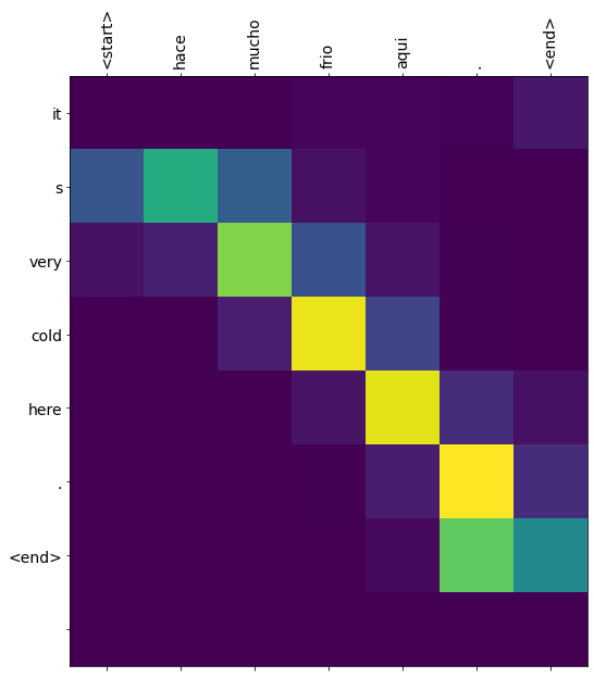
我们可以很清晰地看到模型在翻译过程中注意力的分配。

Reference

• Natural Language Processing with Deep Learning, Stanford University, CS224N, 2019 winter

• https://www.tensorflow.org/tutorials/text/nmt_with_attention

• http://www.manythings.org/anki/