吴恩达机器学习作业1---linear regression

linear regression

文章目录

- - linear regression

1. 代码演示

1.单变量的线性回归

本次作业在jupyter notebook上完成

首先，导入需要用到的类库

import numpy as np
import matplotlib.pyplot as plt
from mpl_toolkits.mplot3d import axes3d, Axes3D
from matplotlib import cm
import itertools

%matplotlib inline

加载文件ex1dara1.txt

datafile = 'data/ex1data1.txt'

#','为分隔符，抽出第0列和第1列，转置
cols = np.loadtxt(datafile,delimiter=',',usecols=(0,1),unpack=True) #Read in comma separated data

#X为第0列，y为第1列
X = np.transpose(np.array(cols[:-1]))
y = np.transpose(np.array(cols[-1:]))
m = y.size 

#在矩阵第一列前加上全为1的一列,目的是1到时候就是常数
X = np.insert(X,0,1,axis=1)

画图看看数据的分布

plt.figure(figsize=(10,6))
plt.plot(X[:,1],y[:,0],'rx',markersize=10)
plt.grid(True) #Always plot.grid true!
plt.ylabel('Profit')
plt.xlabel('Population')

在这里插入图片描述
定义两个函数，一个用于计算线性回归值，一个用于计算损失值

#线性假设函数
def h(theta,X): #Linear hypothesis function
    return np.dot(X,theta)

#利用公式计算损失值
def computeCost(mytheta,X,y): 
    return float((1/(2*m)) * np.dot((h(mytheta,X)-y).T,h(mytheta,X)-y))

定义迭代次数和学习率

iterations = 1500
alpha = 0.01

#测试，返回32.07
test_theta = np.zeros((X.shape[1],1))
print(computeCost(test_theta, X ,y))

定义梯度下降函数

#Actual gradient descent minimizing routine
def descendGradient(X, y, theta_start = np.zeros(2),alpha=0.01,iterations=1500):
    theta = theta_start
    #损失值的列表,len=1500
    costList = []
    #theta值列表,len=1500
    theta_history = []
    for i in range(iterations):
        tmp_theta = theta
        #计算损失值并记录
        costList.append(computeCost(theta,X,y))
        theta_history.append(list(theta[:,0]))
        #同时对每个特征进行更新
        for j in range(len(tmp_theta)):
            tmp_theta[j] = theta[j] - (alpha/m)*np.sum((h(initial_theta,X) - y)*np.array(X[:,j]).reshape(m,1))#梯度下降
        #theta更新
        theta = tmp_theta
    return theta, theta_history, costList

初始化参数，定义绘制cost函数迭代图像的函数

#初始化参数theta
initial_theta = np.zeros((X.shape[1],1))
theta, theta_history, costList = descendGradient(X,y,initial_theta)

#绘制cost值随迭代次数的变化图像
def plotConvergence(costList):
    plt.figure(figsize=(10,6))
    plt.plot(range(len(costList)),costList,'bo')
    plt.grid(True)
    plt.title("Convergence of Cost Function")
    plt.xlabel("Iteration number")
    plt.ylabel("Cost function")
    #设置x，y轴的范围
    plt.xlim([-0.05*iterations,1.05*iterations])
    plt.ylim([4,7])

#测试
plotConvergence(costList)

在这里插入图片描述
绘制拟合曲线图

#Plot the line on top of the data to ensure it looks correct
def myfit(xval):
    return theta[0] + theta[1]*xval

plt.figure(figsize=(10,6))
#绘制红叉散点
plt.plot(X[:,1],y[:,0],'rx',markersize=10,label='Training Data')
#绘制拟合直线
plt.plot(X[:,1],myfit(X[:,1]),'b-',label = 'Hypothesis: h(x) = %0.2f + %0.2fx'%(theta[0],theta[1]))
#添加网格线
plt.grid(True)
plt.ylabel('Profit in $10,000s')
plt.xlabel('Population of City in 10,000s')
plt.legend()

在这里插入图片描述
绘制梯度下降图

fig = plt.figure(figsize=(12,12))
ax = fig.gca(projection='3d')

#设置x，y轴的范围
xvals = np.arange(-10,10,.5)
yvals = np.arange(-1,4,.1)

#设置曲面散点
myxs, myys, myzs = [], [], []
for i in xvals:
    for j in yvals:
        myxs.append(i)
        myys.append(j)
        myzs.append(computeCost(np.array([[i], [j]]),X,y))

#绘制曲面
scat = ax.scatter(myxs,myys,myzs,c=np.abs(myzs),cmap=plt.get_cmap('YlOrRd'))

#添加轴名称
plt.xlabel(r'$\theta_0$',fontsize=30)
plt.ylabel(r'$\theta_1$',fontsize=30)

plt.title('Cost (Minimization Path Shown in Blue)',fontsize=30)
#绘制梯度下降路线
plt.plot([x[0] for x in theta_history],[x[1] for x in theta_history],costList,'bo-')
plt.show()

在这里插入图片描述

2.多元线性回归

加载数据

datafile = 'data/ex1data2.txt'

#cols.shape = (3,47)
cols = np.loadtxt(datafile,delimiter=',',usecols=(0,1,2),unpack=True)

#X前两列,y最后一列
X = np.transpose(np.array(cols[:-1]))
y = np.transpose(np.array(cols[-1:]))
#训练集大小
m = y.size 

#Insert the usual column of 1's into the "X" matrix
X = np.insert(X,0,1,axis=1)

绘制数据分布柱状图

#Quick visualize data

#X每列的数据之间规模相差较大
plt.grid(True)
plt.xlim([-100,5000])

plt.hist(X[:,0],label = 'col1')
plt.hist(X[:,1],label = 'col2')
plt.hist(X[:,2],label = 'col3')

plt.title('Clearly we need feature normalization.')
plt.xlabel('Column Value')
plt.ylabel('Counts')
plt.legend()

在这里插入图片描述
可以看出X的每列数据之间规模相差很大，col1，col2直接消失了

标准化处理X

#标准化处理X
stored_feature_means, stored_feature_stds = [], []
Xnorm = X.copy()
for i in range(Xnorm.shape[1]):
    stored_feature_means.append(np.mean(Xnorm[:,i]))#第i列均值
    stored_feature_stds.append(np.std(Xnorm[:,i]))#第i列标准差
    #跳过第0列
    if not i: continue
    #将数据标准化
    Xnorm[:,i] = (Xnorm[:,i] - stored_feature_means[-1])/stored_feature_stds[-1]

# #标准化处理y
# stored_feature_means, stored_feature_stds = [], []
# ynorm=y.copy()
# for i in range(ynorm.shape[1]):
#     stored_feature_means.append(np.mean(ynorm[:,i]))#第i列均值
#     stored_feature_stds.append(np.std(ynorm[:,i]))#第i列标准差
#     #将数据标准化
#     ynorm[:,i] = (ynorm[:,i] - stored_feature_means[-1])/stored_feature_stds[-1]

再看看数据分布

#Quick visualize the feature-normalized data
plt.grid(True)
plt.xlim([-5,5])
dummy = plt.hist(Xnorm[:,0],label = 'col1')
dummy = plt.hist(Xnorm[:,1],label = 'col2')
dummy = plt.hist(Xnorm[:,2],label = 'col3')

plt.title('Feature Normalization Accomplished')
plt.xlabel('Column Value')
plt.ylabel('Counts')
dummy = plt.legend()

在这里插入图片描述
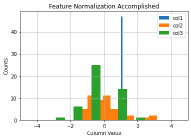
这次就正常了

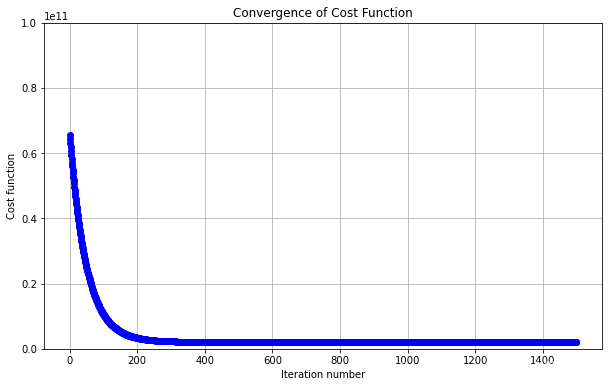
看看cost的迭代拟合情况

#Run gradient descent with multiple variables, initial theta still set to zeros
#(Note! This doesn't work unless we feature normalize! "overflow encountered in multiply")
initial_theta = np.zeros((Xnorm.shape[1],1))
#梯度下降
theta, theta_history, costList = descendGradient(Xnorm, y, initial_theta)
#Plot convergence of cost function:

#因为y值很大，所以cost值很大
plotConvergence(costList)
plt.ylim([0,100000000000])

在这里插入图片描述
训练完成，得到了参数θ，下面进行预测

#训练了线性回归模型，得到了参数θ
#测试预测结果
print ("Check of result: What is price of house with 1650 square feet and 3 bedrooms?")
ytest = np.array([1650.,3.])
#标准化
ytestscaled = [(ytest[x]-stored_feature_means[x+1])/stored_feature_stds[x+1] for x in range(len(ytest))]
ytestscaled.insert(0,1)
print ("$%0.2f" % float(h(theta,ytestscaled)))

Check of result: What is price of house with 1650 square feet and 3 bedrooms?
$293098.15
完成预测

3.Normal equation算法

$\theta=(X^{T}X)^{-1}X^{T}y$

from numpy.linalg import inv
#Implementation of normal equation to find analytic solution to linear regression
def normEqtn(X,y):
    return np.dot(np.dot(inv(np.dot(X.T,X)),X.T),y)

测试一下

print ("Normal equation prediction for price of house with 1650 square feet and 3 bedrooms")
print ("$%0.2f" % float(h(normEqtn(X,y),[1,1650.,3])))

Normal equation prediction for price of house with 1650 square feet and 3 bedrooms
$293081.46

采用梯度下降法得到的预测是 $293098.15
normal equation算法的到的预测是 $293081.46

2. 测试集1

6.1101,17.592
5.5277,9.1302
8.5186,13.662
7.0032,11.854
5.8598,6.8233
8.3829,11.886
7.4764,4.3483
8.5781,12
6.4862,6.5987
5.0546,3.8166
5.7107,3.2522
14.164,15.505
5.734,3.1551
8.4084,7.2258
5.6407,0.71618
5.3794,3.5129
6.3654,5.3048
5.1301,0.56077
6.4296,3.6518
7.0708,5.3893
6.1891,3.1386
20.27,21.767
5.4901,4.263
6.3261,5.1875
5.5649,3.0825
18.945,22.638
12.828,13.501
10.957,7.0467
13.176,14.692
22.203,24.147
5.2524,-1.22
6.5894,5.9966
9.2482,12.134
5.8918,1.8495
8.2111,6.5426
7.9334,4.5623
8.0959,4.1164
5.6063,3.3928
12.836,10.117
6.3534,5.4974
5.4069,0.55657
6.8825,3.9115
11.708,5.3854
5.7737,2.4406
7.8247,6.7318
7.0931,1.0463
5.0702,5.1337
5.8014,1.844
11.7,8.0043
5.5416,1.0179
7.5402,6.7504
5.3077,1.8396
7.4239,4.2885
7.6031,4.9981
6.3328,1.4233
6.3589,-1.4211
6.2742,2.4756
5.6397,4.6042
9.3102,3.9624
9.4536,5.4141
8.8254,5.1694
5.1793,-0.74279
21.279,17.929
14.908,12.054
18.959,17.054
7.2182,4.8852
8.2951,5.7442
10.236,7.7754
5.4994,1.0173
20.341,20.992
10.136,6.6799
7.3345,4.0259
6.0062,1.2784
7.2259,3.3411
5.0269,-2.6807
6.5479,0.29678
7.5386,3.8845
5.0365,5.7014
10.274,6.7526
5.1077,2.0576
5.7292,0.47953
5.1884,0.20421
6.3557,0.67861
9.7687,7.5435
6.5159,5.3436
8.5172,4.2415
9.1802,6.7981
6.002,0.92695
5.5204,0.152
5.0594,2.8214
5.7077,1.8451
7.6366,4.2959
5.8707,7.2029
5.3054,1.9869
8.2934,0.14454
13.394,9.0551
5.4369,0.61705

3. 测试集2

2104,3,399900
1600,3,329900
2400,3,369000
1416,2,232000
3000,4,539900
1985,4,299900
1534,3,314900
1427,3,198999
1380,3,212000
1494,3,242500
1940,4,239999
2000,3,347000
1890,3,329999
4478,5,699900
1268,3,259900
2300,4,449900
1320,2,299900
1236,3,199900
2609,4,499998
3031,4,599000
1767,3,252900
1888,2,255000
1604,3,242900
1962,4,259900
3890,3,573900
1100,3,249900
1458,3,464500
2526,3,469000
2200,3,475000
2637,3,299900
1839,2,349900
1000,1,169900
2040,4,314900
3137,3,579900
1811,4,285900
1437,3,249900
1239,3,229900
2132,4,345000
4215,4,549000
2162,4,287000
1664,2,368500
2238,3,329900
2567,4,314000
1200,3,299000
852,2,179900
1852,4,299900
1203,3,239500