目录
参考Pandas官方文档,Pandas快速教程,供自己复习使用。
一.概览
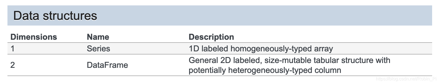
1. 两大数据结构:Series和DateFrame(分别对应一维数据和二维数据)
2. NumPy和Pandas的本质差别
a fundamental difference between pandas and NumPy: NumPy arrays have one dtype for the entire array, while pandas DataFrames have one dtype per column.
即NumPy数组中的数据元素只能有一种数据类型,而Pandas DateFrame的每一列(分别)都可以有一种。
3. 记住:
index(the rows) 用来代替 axis=0;
columns 用来代替axis=1
二.快速入门
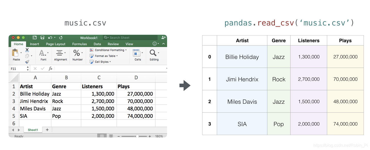
1. 数据导入
- CSV文件、Excel文件、HDF5
pd.read_csv()
pd.read_excel()
pd.read_hdf()
df = pandas.read_csv('music.csv')
2. 查看数据(Viewing Data)
-
df.head() 查看头
-
df.tail() 查看尾
-
df.index() 查看索引
-
df.column() 查看列名
-
df.to_numpy() 展示底层数据的NumPy数组表示
-
df.describe() 查看数据的一些统计数据,比如计数、平均值、最大值等等:
-
df.T 转置数据
-
df.sort_index() 按轴排序
-
df.sort_values() 按值排序
3. 选择(Selection)
Pandas中有 df[ ]、df.X ; df.loc[ ] 、 df.iloc[ ] ; .at[ ]、.iat[ ] 等数据访问方法。
3.1 df[ ]、df.X
① 选择单列,df[ X ]、df.X两种方式等价
In [23]: df['A']
Out[23]:
2013-01-01    0.469112
2013-01-02    1.212112
2013-01-03   -0.861849
2013-01-04    0.721555
2013-01-05   -0.424972
2013-01-06   -0.673690
Freq: D, Name: A, dtype: float64
② df[ ]可以使用切片获取多行数据
In [24]: df[0:3]
Out[24]:
                   A         B         C         D
2013-01-01  0.469112 -0.282863 -1.509059 -1.135632
2013-01-02  1.212112 -0.173215  0.119209 -1.044236
2013-01-03 -0.861849 -2.104569 -0.494929  1.071804

In [25]: df['20130102':'20130104']
Out[25]:
                   A         B         C         D
2013-01-02  1.212112 -0.173215  0.119209 -1.044236
2013-01-03 -0.861849 -2.104569 -0.494929  1.071804
2013-01-04  0.721555 -0.706771 -1.039575  0.271860
3.2 df.loc[ ]
df.loc[ ]通过使用标签(列目录)来获得列数据、行数据
① df.loc[ ] 使用切片,提取(全行)一列或者(全行)多列数据
In [26]: df.loc[dates[0]]  # 一列数据
Out[26]:
A    0.469112
B   -0.282863
C   -1.509059
D   -1.135632
Name: 2013-01-01 00:00:00, dtype: float64
In [27]: df.loc[:, ['A', 'B']]  # 多列数据
Out[27]:
                   A         B
2013-01-01  0.469112 -0.282863
2013-01-02  1.212112 -0.173215
2013-01-03 -0.861849 -2.104569
2013-01-04  0.721555 -0.706771
2013-01-05 -0.424972  0.567020
2013-01-06 -0.673690  0.113648
② df.loc[ ] 提取多行和多列数据(切片)
In [28]: df.loc['20130102':'20130104', ['A', 'B']]
Out[28]:
                   A         B
2013-01-02  1.212112 -0.173215
2013-01-03 -0.861849 -2.104569
2013-01-04  0.721555 -0.706771
③ df.loc[ ] 提取单行多列数据
In [29]: df.loc['20130102', ['A', 'B']] # 实现了降维
Out[29]:
A    1.212112
B   -0.173215
Name: 2013-01-02 00:00:00, dtype: float64
In [30]: df.loc[dates[0], 'A']  # 提取单个数据
Out[30]: 0.46911229990718628
思考:选取列数据,比如‘A’ 时 ,df.loc[ : , ‘A’ ]、df[ ‘A’ ] 、df.A这三种方法是一样的么?
loc的方法更强大,可以同时涉及行和列
参考:http://www.ojit.com/article/85145
3.3 df.iloc[ ]
df.iloc[ ] 通过使用位置(索引)来进行数据选择,类似NumPy和Python。
① df.iloc[ ]用整数(按位置)选择某一行数据
In [32]: df.iloc[3]
Out[32]:
A    0.721555
B   -0.706771
C   -1.039575
D    0.271860
Name: 2013-01-04 00:00:00, dtype: float64
② df.iloc[ ]用整数切片(按位置)来获取多行多列数据
In [33]: df.iloc[3:5, 0:2]
Out[33]:
                   A         B
2013-01-04  0.721555 -0.706771
2013-01-05 -0.424972  0.567020
③ df.iloc[ ]用整数列表(按位置)来获取多行多列数据
In [34]: df.iloc[[1, 2, 4], [0, 2]]
Out[34]:
                   A         C
2013-01-02  1.212112  0.119209
2013-01-03 -0.861849 -0.494929
2013-01-05 -0.424972  0.276232
④ df.iloc[ ] 用:(按位置)获取整行/列切片数据
In [35]: df.iloc[1:3, :]
Out[35]:
                   A         B         C         D
2013-01-02  1.212112 -0.173215  0.119209 -1.044236
2013-01-03 -0.861849 -2.104569 -0.494929  1.071804
In [36]: df.iloc[:, 1:3]
Out[36]:
                   B         C
2013-01-01 -0.282863 -1.509059
2013-01-02 -0.173215  0.119209
2013-01-03 -2.104569 -0.494929
2013-01-04 -0.706771 -1.039575
2013-01-05  0.567020  0.276232
2013-01-06  0.113648 -1.478427
⑤ df.iloc[ ] (按位置)提取单个数据
In [37]: df.iloc[1, 1]
Out[37]: -0.17321464905330858
4.过滤
使用>、<、==等布尔索引进行数据过滤。
In [39]: df[df.A > 0]
Out[39]:
                   A         B         C         D
2013-01-01  0.469112 -0.282863 -1.509059 -1.135632
2013-01-02  1.212112 -0.173215  0.119209 -1.044236
2013-01-04  0.721555 -0.706771 -1.039575  0.271860
In [40]: df[df > 0]
Out[40]:
                   A         B         C         D
2013-01-01  0.469112       NaN       NaN       NaN
2013-01-02  1.212112       NaN  0.119209       NaN
2013-01-03       NaN       NaN       NaN  1.071804
2013-01-04  0.721555       NaN       NaN  0.271860
2013-01-05       NaN  0.567020  0.276232       NaN
2013-01-06       NaN  0.113648       NaN  0.524988
In [41]: df2 = df.copy()

In [42]: df2['E'] = ['one', 'one', 'two', 'three', 'four', 'three']

In [43]: df2
Out[43]:
                   A         B         C         D      E
2013-01-01  0.469112 -0.282863 -1.509059 -1.135632    one
2013-01-02  1.212112 -0.173215  0.119209 -1.044236    one
2013-01-03 -0.861849 -2.104569 -0.494929  1.071804    two
2013-01-04  0.721555 -0.706771 -1.039575  0.271860  three
2013-01-05 -0.424972  0.567020  0.276232 -1.087401   four
2013-01-06 -0.673690  0.113648 -1.478427  0.524988  three

In [44]: df2[df2['E'].isin(['two', 'four'])]
Out[44]:
                   A         B         C         D     E
2013-01-03 -0.861849 -2.104569 -0.494929  1.071804   two
2013-01-05 -0.424972  0.567020  0.276232 -1.087401  four
5. 设值(Setting)
通过赋值增加新的列到原数据。
其基本操作跟”获取“数据的操作一致。
In [45]: s1 = pd.Series([1, 2, 3, 4, 5, 6], index=pd.date_range('20130102', periods=6))

In [46]: s1
Out[46]:
2013-01在这里插入代码片-02    1
2013-01-03    2
2013-01-04    3
2013-01-05    4
2013-01-06    5
2013-01-07    6
Freq: D, dtype: int64

In [47]: df['F'] = s1
按标签赋值:
In [48]: df.at[dates[0], 'A'] = 0
按位置赋值:
In [49]: df.iat[0, 1] = 0
按NumPy数组赋值:
In [50]: df.loc[:, 'D'] = np.array([5] * len(df))
使用设值(Setting)的一个where 操作:
In [52]: df2 = df.copy()

In [53]: df2[df2 > 0] = -df2

In [54]: df2
Out[54]:
                   A         B         C  D    F
2013-01-01  0.000000  0.000000 -1.509059 -5  NaN
2013-01-02 -1.212112 -0.173215 -0.119209 -5 -1.0
2013-01-03 -0.861849 -2.104569 -0.494929 -5 -2.0
2013-01-04 -0.721555 -0.706771 -1.039575 -5 -3.0
2013-01-05 -0.424972 -0.567020 -0.276232 -5 -4.0
2013-01-06 -0.673690 -0.113648 -1.478427 -5 -5.0
6. 缺失值(Missing data)
Pandas 主要使用 np.nan 来表示缺失的数据。 进行运算时,默认不包含空值。
- 如何开始
使用reindex可以增加、删除和更改指定轴的索引,并返回数据的副本,即不改变原来的数据。(不同于NumPy的resize操作)
In [55]: df1 = df.reindex(index=dates[0:4], columns=list(df.columns) + ['E'])

In [56]: df1.loc[dates[0]:dates[1], 'E'] = 1

In [57]: df1
Out[57]:
                   A         B         C  D    F    E
2013-01-01  0.000000  0.000000 -1.509059  5  NaN  1.0
2013-01-02  1.212112 -0.173215  0.119209  5  1.0  1.0
2013-01-03 -0.861849 -2.104569 -0.494929  5  2.0  NaN
2013-01-04  0.721555 -0.706771 -1.039575  5  3.0  NaN
- 删除含有缺失值的行
df.dropna( )
In [58]: df1.dropna(how='any')
Out[58]:
                   A         B         C  D    F    E
2013-01-02  1.212112 -0.173215  0.119209  5  1.0
- 填充缺失值
df.fillna( )
In [59]: df1.fillna(value=5)
Out[59]:
                   A         B         C  D    F    E
2013-01-01  0.000000  0.000000 -1.509059  5  5.0  1.0
2013-01-02  1.212112 -0.173215  0.119209  5  1.0  1.0
2013-01-03 -0.861849 -2.104569 -0.494929  5  2.0  5.0
2013-01-04  0.721555 -0.706771 -1.039575  5  3.0  5.0
- 根据是否含缺失值来取布尔掩码
pd.isna( )
In [60]: pd.isna(df1)
Out[60]:
                A      B      C      D      F      E
2013-01-01  False  False  False  False   True  False
2013-01-02  False  False  False  False  False  False
2013-01-03  False  False  False  False  False   True
2013-01-04  False  False  False  False  False   True
7. 运算(Operations)
- 统计
运算一般将缺失值排除在外。
一般的聚合(aggregation)函数包括 mean()、min() 和 max() 等。
In [61]: df.mean()
Out[61]:
A   -0.004474
B   -0.383981
C   -0.687758
D    5.000000
F    3.000000
dtype: float64
可以在另外一个轴(行——列变化)上进行相同操作:
In [62]: df.mean(1)
Out[62]:
2013-01-01    0.872735
2013-01-02    1.431621
2013-01-03    0.707731
2013-01-04    1.395042
2013-01-05    1.883656
2013-01-06    1.592306
Freq: D, dtype: float64
- Apply函数
In [66]: df.apply(np.cumsum)
Out[66]:
                   A         B         C   D     F
2013-01-01  0.000000  0.000000 -1.509059   5   NaN
2013-01-02  1.212112 -0.173215 -1.389850  10   1.0
2013-01-03  0.350263 -2.277784 -1.884779  15   3.0
2013-01-04  1.071818 -2.984555 -2.924354  20   6.0
2013-01-05  0.646846 -2.417535 -2.648122  25  10.0
2013-01-06 -0.026844 -2.303886 -4.126549  30  15.0

In [67]: df.apply(lambda x: x.max() - x.min())
Out[67]:
A    2.073961
B    2.671590
C    1.785291
D    0.000000
F    4.000000
dtype: float64
- 直方图
In [68]: s = pd.Series(np.random.randint(0, 7, size=10))

In [69]: s
Out[69]:
0    4
1    2
2    1
3    2
4    6
5    4
6    4
7    6
8    4
9    4
dtype: int64

In [70]: s.value_counts()
Out[70]:
4    5
6    2
2    2
1    1
dtype: int64
- 字符串方法
In [71]: s = pd.Series(['A', 'B', 'C', 'Aaba', 'Baca', np.nan, 'CABA', 'dog', 'cat'])

In [72]: s.str.lower()
Out[72]:
0       a
1       b
2       c
3    aaba
4    baca
5     NaN
6    caba
7     dog
8     cat
dtype: object
8. 合并(Merge)
8.1 concat()
In [73]: df = pd.DataFrame(np.random.randn(10, 4))

In [74]: df
Out[74]:
          0         1         2         3
0 -0.548702  1.467327 -1.015962 -0.483075
1  1.637550 -1.217659 -0.291519 -1.745505
2 -0.263952  0.991460 -0.919069  0.266046
3 -0.709661  1.669052  1.037882 -1.705775
4 -0.919854 -0.042379  1.247642 -0.009920
5  0.290213  0.495767  0.362949  1.548106
6 -1.131345 -0.089329  0.337863 -0.945867
7 -0.932132  1.956030  0.017587 -0.016692
8 -0.575247  0.254161 -1.143704  0.215897
9  1.193555 -0.077118 -0.408530 -0.862495

# 分解为多组
In [75]: pieces = [df[:3], df[3:7], df[7:]]

In [76]: pd.concat(pieces)
Out[76]:
          0         1         2         3
0 -0.548702  1.467327 -1.015962 -0.483075
1  1.637550 -1.217659 -0.291519 -1.745505
2 -0.263952  0.991460 -0.919069  0.266046
3 -0.709661  1.669052  1.037882 -1.705775
4 -0.919854 -0.042379  1.247642 -0.009920
5  0.290213  0.495767  0.362949  1.548106
6 -1.131345 -0.089329  0.337863 -0.945867
7 -0.932132  1.956030  0.017587 -0.016692
8 -0.575247  0.254161 -1.143704  0.215897
9  1.193555 -0.077118 -0.408530 -0.862495
8.2 merg():连接(Join)
In [77]: left = pd.DataFrame({

    'key': ['foo', 'foo'], 'lval': [1, 2]})

In [78]: right = pd.DataFrame({

    'key': ['foo', 'foo'], 'rval': [4, 5]})

In [79]: left
Out[79]:
   key  lval
0  foo     1
1  foo     2

In [80]: right
Out[80]:
   key  rval
0  foo     4
1  foo     5

In [81]: pd.merge(left, right, on='key')
Out[81]:
   key  lval  rval
0  foo     1     4
1  foo     1     5
2  foo     2     4
3  foo     2     5
另外一个例子:
In [82]: left = pd.DataFrame({

    'key': ['foo', 'bar'], 'lval': [1, 2]})

In [83]: right = pd.DataFrame({

    'key': ['foo', 'bar'], 'rval': [4, 5]})

In [84]: left
Out[84]:
   key  lval
0  foo     1
1  bar     2

In [85]: right
Out[85]:
   key  rval
0  foo     4
1  bar     5

In [86]: pd.merge(left, right, on='key')
Out[86]:
   key  lval  rval
0  foo     1     4
1  bar     2     5
8.3 append():追加(Append)
In [87]: df = pd.DataFrame(np.random.randn(8, 4), columns=['A', 'B', 'C', 'D'])

In [88]: df
Out[88]:
          A         B         C         D
0  1.346061  1.511763  1.627081 -0.990582
1 -0.441652  1.211526  0.268520  0.024580
2 -1.577585  0.396823 -0.105381 -0.532532
3  1.453749  1.208843 -0.080952 -0.264610
4 -0.727965 -0.589346  0.339969 -0.693205
5 -0.339355  0.593616  0.884345  1.591431
6  0.141809  0.220390  0.435589  0.192451
7 -0.096701  0.803351  1.715071 -0.708758

In [89]: s = df.iloc[3]

In [90]: df.append(s, ignore_index=True)
Out[90]:
          A         B         C         D
0  1.346061  1.511763  1.627081 -0.990582
1 -0.441652  1.211526  0.268520  0.024580
2 -1.577585  0.396823 -0.105381 -0.532532
3  1.453749  1.208843 -0.080952 -0.264610
4 -0.727965 -0.589346  0.339969 -0.693205
5 -0.339355  0.593616  0.884345  1.591431
6  0.141809  0.220390  0.435589  0.192451
7 -0.096701  0.803351  1.715071 -0.708758
8  1.453749  1.208843 -0.080952 -0.264610
8. 分组(Grouping)
分组有以下一项或多项步骤的处理流程:
分割:根据需求将数据分组;
函数:将函数分别应用到每个组;
结合:将得到的结果组成一个新的数据结构;
In [91]: df = pd.DataFrame({

    'A': ['foo', 'bar', 'foo', 'bar',
   ....:                          'foo', 'bar', 'foo', 'foo'],
   ....:                    'B': ['one', 'one', 'two', 'three',
   ....:                          'two', 'two', 'one', 'three'],
   ....:                    'C': np.random.randn(8),
   ....:                    'D': np.random.randn(8)})
   ....:

In [92]: df
Out[92]:
     A      B         C         D
0  foo    one -1.202872 -0.055224
1  bar    one -1.814470  2.395985
2  foo    two  1.018601  1.552825
3  bar  three -0.595447  0.166599
4  foo    two  1.395433  0.047609
5  bar    two -0.392670 -0.136473
6  foo    one  0.007207 -0.561757
7  foo  three  1.928123 -1.623033
分组+应用函数:
In [93]: df.groupby('A').sum()
Out[93]:
            C        D
A
bar -2.802588  2.42611
foo  3.146492 -0.63958
分组为多层索引+应函数:
In [94]: df.groupby(['A', 'B']).sum()
Out[94]:
                  C         D
A   B
bar one   -1.814470  2.395985
    three -0.595447  0.166599
    two   -0.392670 -0.136473
foo one   -1.195665 -0.616981
    three  1.928123 -1.623033
    two    2.414034  1.600434
9. 重塑(Reshaping)
堆叠(Stack)
In [95]: tuples = list(zip(*[['bar', 'bar', 'baz', 'baz',
   ....:                      'foo', 'foo', 'qux', 'qux'],
   ....:                     ['one', 'two', 'one', 'two',
   ....:                      'one', 'two', 'one', 'two']]))
   ....:

In [96]: index = pd.MultiIndex.from_tuples(tuples, names=['first', 'second'])

In [97]: df = pd.DataFrame(np.random.randn(8, 2), index=index, columns=['A', 'B'])

In [98]: df2 = df[:4]

In [99]: df2
Out[99]:
                     A         B
first second
bar   one     0.029399 -0.542108
      two     0.282696 -0.087302
baz   one    -1.575170  1.771208
      two     0.816482  1.100230
stack() 方法把 DataFrame 列压缩至一层:
In [100]: stacked = df2.stack()

In [101]: stacked
Out[101]:
first  second
               B   -0.542108
       two     A    0.282696
               B   -0.087302
baz    one     A   -1.575170
               B    1.771208
       two     A    0.816482
               B    1.100230
dtype: float64
压缩后(stacked)的 DataFrame 或 Series 具有多层索引, stack() 的逆操作是 unstack() ,默认拆叠最后一层:
In [102]: stacked.unstack()
Out[102]:
                     A         B
first second
bar   one     0.029399 -0.542108
      two     0.282696 -0.087302
baz   one    -1.575170  1.771208
      two     0.816482  1.100230

In [103]: stacked.unstack(1)
Out[103]:
second        one       two
first
bar   A  0.029399  0.282696
      B -0.542108 -0.087302
baz   A -1.575170  0.816482
      B  1.771208  1.100230

In [104]: stacked.unstack(0)
Out[104]:
first          bar       baz
second
one    A  0.029399 -1.575170
       B -0.542108  1.771208
two    A  0.282696  0.816482
       B -0.087302  1.100230
10. 透视图(Pivot tables)
In [105]: df = pd.DataFrame({

    'A': ['one', 'one', 'two', 'three'] * 3,
   .....:                    'B': ['A', 'B', 'C'] * 4,
   .....:                    'C': ['foo', 'foo', 'foo', 'bar', 'bar', 'bar'] * 2,
   .....:                    'D': np.random.randn(12),
   .....:                    'E': np.random.randn(12)})
   .....:

In [106]: df
Out[106]:
        A  B    C         D         E
0     one  A  foo  1.418757 -0.179666
1     one  B  foo -1.879024  1.291836
2     two  C  foo  0.536826 -0.009614
3   three  A  bar  1.006160  0.392149
4     one  B  bar -0.029716  0.264599
5     one  C  bar -1.146178 -0.057409
6     two  A  foo  0.100900 -1.425638
7   three  B  foo -1.035018  1.024098
8     one  C  foo  0.314665 -0.106062
9     one  A  bar -0.773723  1.824375
10    two  B  bar -1.170653  0.595974
11  three  C  bar  0.648740  1.167115
很容易就能生成透视图:
In [107]: pd.pivot_table(df, values='D', index=['A', 'B'], columns=['C'])
Out[107]:
C             bar       foo
A     B
one   A -0.773723  1.418757
      B -0.029716 -1.879024
      C -1.146178  0.314665
three A  1.006160       NaN
      B       NaN -1.035018
      C  0.648740       NaN
two   A       NaN  0.100900
      B -1.170653       NaN
      C       NaN  0.536826
11. 时间序列(Time series)、类别型(Categoricals)、Ploting(可视化)、数据输出(Getting data out)暂略
写在最后
思考:
对于这些知识点的罗列,顶多算知道了Pandas是什么,有哪些东西在里面——“what”,
但是离如何使用还有一段距离,因此要学会如何去使用Pandas——“How”,但是在这之前不妨想一想,为什么会有Pandas出现?大家都拿他来干些什么?——“Why”。
刚好,昨天刚买的书到了,有这样一段话,对我这个数据分析小白来说有些启发,在此记录一下:
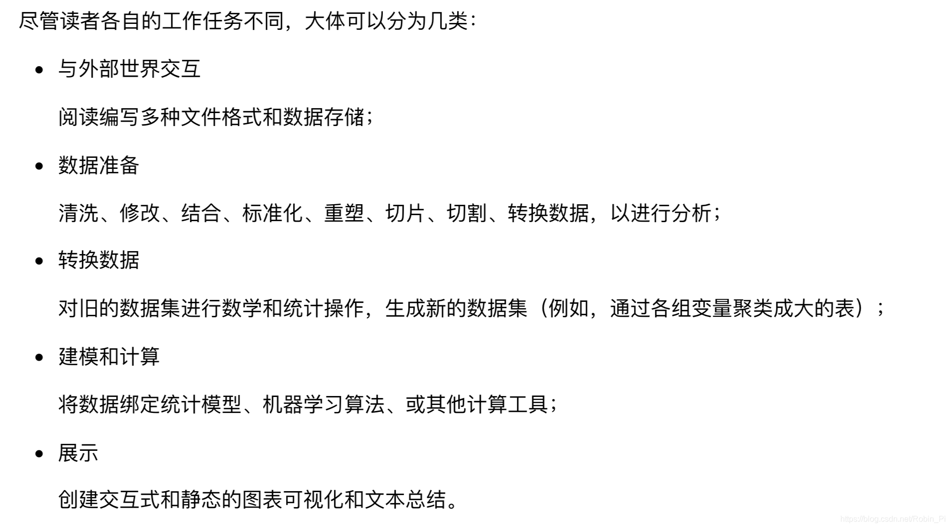 归根到底,我们所做的一切事情,在本质上,不过是将现实生活里的事物的一些记录和规律(数据),转变成计算机能够接受的方式(向量);在此基础上我们进一步处理这些数据,“取其精华去其糟粕”,从中找出我们需要的部分组成新的数据;接着,再将这些已经向量化的数据的格式进行调整,并将其输送到计算机中的数学模型中,进行模型训练;我们不断地调整模型并输出最后的结果,最后我们得以可视化我们的结果。