2.Related Work
Image Compression
- Progressively encodes the image using a recurrent neural network
allow for variable compression rates with a single model - Use fully convolutional networks to handle arbitrary image sizes
Bottleneck:contains spatially redundant activations
Entropy coding further compresses this redundant information - Learning the binary representation is inherently non-differentiable
- Stochastic binarization and backpropagate
- soft assignment to approximate quantization
- replace the quantization by adding uniform
allow for gradients to flow through the discretization
use stochastic binarization
Video Compression
Two simple ideas:
- Decompose each frame into blocks of pixels, known as macroblocks
Divide frames into image (I) frames and referencing (P or B) frames
I-frames directly compress video frames using image compression.
Most of the savings in video codecs come from referencing frames.
P-frames borrow color values from preceding frames. save motion estimate and a highly compressible difference image for each macroblock.
B-frames additionally allow bidirectional referencing, as long as there are no circular references.
A hierarchical way
I-frames form the top of the hierarchy.
In each consecutive level, P- or B-frames reference decoded frames at higher levels.
The author’s that referencing (P or B) frames are a special case of image interpolation.
Image interpolation and extrapolation
Image interpolation
hallucinate an unseen frame between two reference frames -------> an encoder-decoder network architecture to move pixels through time
- a spatially-varying convolution kernel
- a flow field
- combine two predictions
Image extrapolation
predicts a future video from a few frames, or a still image
The authors’ extend image interpolation and incorporate few compressible bits of side information to reconstruct the original video.
3. Preliminary
\(I^{(t)}\in {R^{WH3}}\) a serires of frames for \(t\in{0,1,…}\)
Goal: compress each frame \(I^{(t)}\) into a binary code \(b^{(t)}\in {
{0,1}}^{N_t}\)
An Encoder E ; A decoder D. E and D have two competing aims:
Minimize the total bitrate \(\sum_{t}N_t\)
Reconstruct the original video as faithfully as possible, measured by \(l(\hat{I},I) = ||\hat{I} - I||_1\)
Image compression
The simplest encoders and decoders process each image independently.
\(E_I:I^{(t)}\to b^{(t)}\)
\(D_t:b^{(t)}\to I^{(t)}\)
Model of Toderici
encodes and reconstructs an image progressively over K iterations. At each iteration, the model encodes a residual \(r_k\) between the previously coded image and the original frame:
\(r_0:=I\)
\(b_k := E_I(r_{k-1},g_{k-1}), r_k := r_{k-1}-D_I(b_k,h_{k-1}), for k 1,2,…\)
\(g_k\)and \(h_k\) are latent Conv-LSTM states that are updated at each iteration. All iterations share the same network architecture and parameters forming a recurrent structure.
The training objective minimizes the distortion at all the steps \(\sum_{k=1}^{K}||r_k||1\)
The reconstructs \(\hat I_K = \sum{k=1}^{K}D_I(b_k)\)
Both the encoder and the decoder consist of 4 Conv-LSTMs with stride 2.
Bottleneck: a binary feature map with L channels and 16 times smaller spatial resolution in both width and height.
Solution Toderici use a stochastic binarization
Video compression
Process I-frames using an image encoder \(E_I\) and decoder \(D_I\)
P-frames store a block motion estimate \(T ∈ R^{W×H×2}\)
The original color frame is then recovered by
I i ( t ) = i i − T i ( t ) ( t − 1 ) + R i ( t ) I_i^{(t)} = i_{i-T_i^{(t)}}^{(t-1)+R_i^{(t)}} Ii(t)=ii−Ti(t)(t−1)+Ri(t)
for every pixel i in the image.
The compression is uniquely defined by a block structure and motion estimate T.
The author’s image interpolation network with motion information and add a compressible bottleneck layer.
4.Video Compression through Interpolation
Chose every n-th frame as an I-frame.
The remaining n − 1 frames are interpolated. R-frames
Basic interpolation network \(\to\) a hierarchical interpolation (reduce the bitrate)
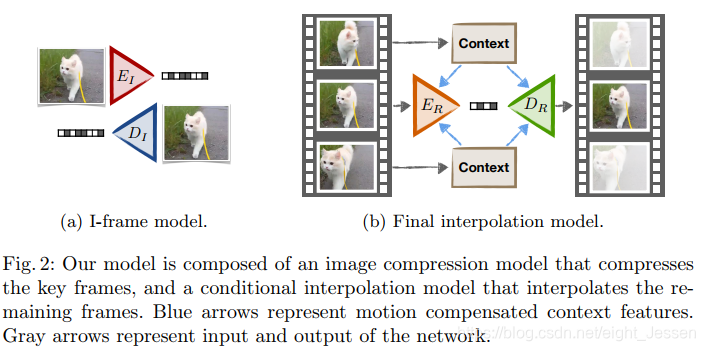
4.1 Interpolation network
A context network \(C:I \to {f{(1)},f{(2)},…}\) to extract a series of feature maps \(f^{(l)}\) of various spatial resolutions
let \(f := {f{(1)},f{(2)},…}\) be the collection of all context features
use the upconvolutional feature maps of a U-net architecture with increasing spatial resolution
C and D are trained jointly.
Motion compensated interpolation
Tried both optical flow and block motion estimation.
Use the motion information to warp each context feature map: \(\check f_i^{(l)} = f_{i-T_i}^{(l)}\) at every spatial location i.
scale the motion estimation with the resolution of the feature map
use bilinear interpolation for fractional locations
drawback: only produces content seen in either reference image. Variations beyond motion, such as change in lighting, deformation,
occlusion, etc. are not captured by this model.
Residual motion compensated interpolation
jointly train an encoder \(E_R\), context model C and interpolation netowrk \(D_R\)
The encoder sees the same information as the interpolation network, which allows it to compress just the missing information, and avoid a redundant encoding.
\(r_0 := I\)
\(b_k := E_R(r_{k-1}, \check f_1,\check f_2,g_{k-1})\)
\(r_k := r_{k-1} - D_R(b_k,\check f_1,\check f_2,h_{k-1})\) for k = 1,2,…
Allows for learning a variable rate compression
4.2 Hierarchical interpolation
maximizing the number of temporally close interpolations
4.3 Implementation
Architecture:
- Toderici Image compression model
- U-net context model
reduce the number of channels of all filters by half
remove the final output layer and takes the feature maps at the resolutions that are 2×, 4×, 8× smaller than the original input image.
Conditional encoder and decoder
fuse the U-net features with the individual Conv-LSTM layers
Entropy coding
Motion compression