机器学习——基础算法(十一)
一、二项分布的最大似然估计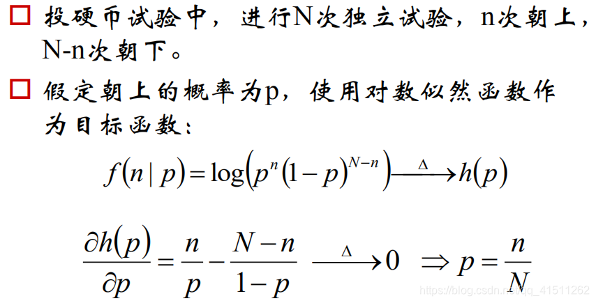
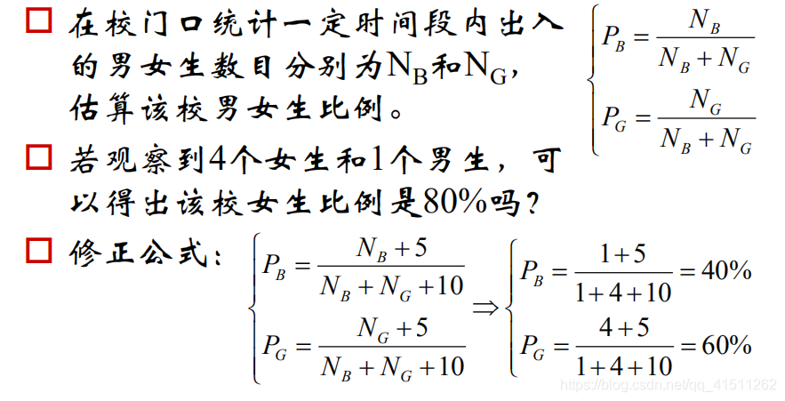
二、二项分布与先验举例
三、EM算法
import numpy as np
from scipy.stats import multivariate_normal
from sklearn.mixture import GaussianMixture
from mpl_toolkits.mplot3d import Axes3D
import matplotlib as mpl
import matplotlib.pyplot as plt
from sklearn.metrics.pairwise import pairwise_distances_argmin
mpl.rcParams['font.sans-serif'] = [u'SimHei']
mpl.rcParams['axes.unicode_minus'] = False
if __name__ == '__main__':
style = 'myself'
np.random.seed(0)
mu1_fact = (0, 0, 0)
cov1_fact = np.diag((1, 2, 3))
data1 = np.random.multivariate_normal(mu1_fact, cov1_fact, 400)
mu2_fact = (2, 2, 1)
cov2_fact = np.array(((1, 1, 3), (1, 2, 1), (0, 0, 1)))
data2 = np.random.multivariate_normal(mu2_fact, cov2_fact, 100)
data = np.vstack((data1, data2))
y = np.array([True] * 400 + [False] * 100)
if style == 'sklearn':
g = GaussianMixture(n_components=2, covariance_type='full', tol=1e-6, max_iter=1000)
g.fit(data)
print ('类别概率:\t', g.weights_[0])
print ('均值:\n', g.means_, '\n')
print ('方差:\n', g.covariances_, '\n')
mu1, mu2 = g.means_
sigma1, sigma2 = g.covariances_
else:
num_iter = 100
n, d = data.shape
# 随机指定
# mu1 = np.random.standard_normal(d)
# print mu1
# mu2 = np.random.standard_normal(d)
# print mu2
mu1 = data.min(axis=0)
mu2 = data.max(axis=0)
sigma1 = np.identity(d)
sigma2 = np.identity(d)
pi = 0.5
# EM
for i in range(num_iter):
# E Step
norm1 = multivariate_normal(mu1, sigma1)
norm2 = multivariate_normal(mu2, sigma2)
tau1 = pi * norm1.pdf(data)
tau2 = (1 - pi) * norm2.pdf(data)
gamma = tau1 / (tau1 + tau2)
# M Step
mu1 = np.dot(gamma, data) / np.sum(gamma)
mu2 = np.dot((1 - gamma), data) / np.sum((1 - gamma))
sigma1 = np.dot(gamma * (data - mu1).T, data - mu1) / np.sum(gamma)
sigma2 = np.dot((1 - gamma) * (data - mu2).T, data - mu2) / np.sum(1 - gamma)
pi = np.sum(gamma) / n
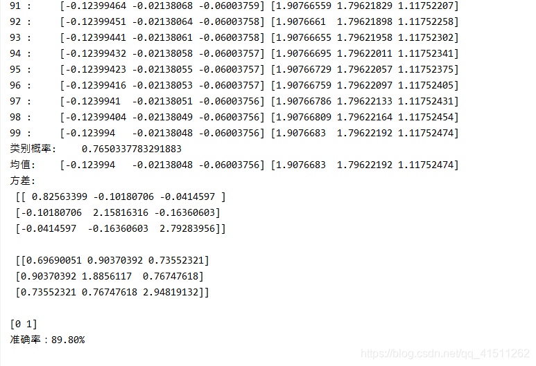
print (i, ":\t", mu1, mu2)
print ('类别概率:\t', pi)
print ('均值:\t', mu1, mu2)
print ('方差:\n', sigma1, '\n\n', sigma2, '\n')
# 预测分类
norm1 = multivariate_normal(mu1, sigma1)
norm2 = multivariate_normal(mu2, sigma2)
tau1 = norm1.pdf(data)
tau2 = norm2.pdf(data)
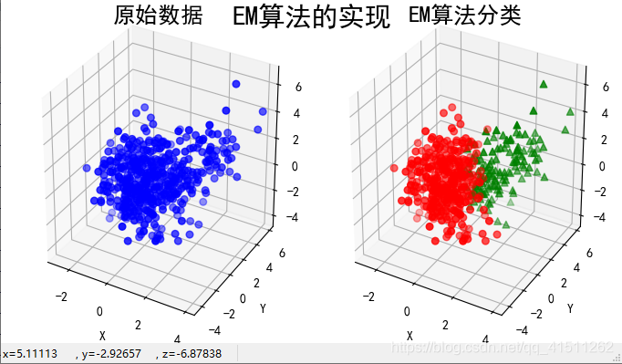
fig = plt.figure(figsize=(13, 7), facecolor='w')
ax = fig.add_subplot(121, projection='3d')
ax.scatter(data[:, 0], data[:, 1], data[:, 2], c='b', s=30, marker='o', depthshade=True)
ax.set_xlabel('X')
ax.set_ylabel('Y')
ax.set_zlabel('Z')
ax.set_title(u'原始数据', fontsize=18)
ax = fig.add_subplot(122, projection='3d')
order = pairwise_distances_argmin([mu1_fact, mu2_fact], [mu1, mu2], metric='euclidean')
print (order)
if order[0] == 0:
c1 = tau1 > tau2
else:
c1 = tau1 < tau2
c2 = ~c1
acc = np.mean(y == c1)
print (u'准确率:%.2f%%' % (100*acc))
ax.scatter(data[c1, 0], data[c1, 1], data[c1, 2], c='r', s=30, marker='o', depthshade=True)
ax.scatter(data[c2, 0], data[c2, 1], data[c2, 2], c='g', s=30, marker='^', depthshade=True)
ax.set_xlabel('X')
ax.set_ylabel('Y')
ax.set_zlabel('Z')
ax.set_title(u'EM算法分类', fontsize=18)
plt.suptitle(u'EM算法的实现', fontsize=21)
plt.subplots_adjust(top=0.90)
plt.tight_layout()
plt.show()
结果截图:
三、GMM算法
import numpy as np
from sklearn.mixture import GaussianMixture
from sklearn.model_selection import train_test_split
import matplotlib as mpl
import matplotlib.colors
import matplotlib.pyplot as plt

mpl.rcParams['font.sans-serif'] = [u'SimHei']
mpl.rcParams['axes.unicode_minus'] = False
# from matplotlib.font_manager import FontProperties
# font_set = FontProperties(fname=r"c:\windows\fonts\simsun.ttc", size=15)
# fontproperties=font_set


def expand(a, b):
    d = (b - a) * 0.05
    return a-d, b+d


if __name__ == '__main__':
    data = np.loadtxt('HeightWeight.csv', dtype=np.float, delimiter=',', skiprows=1)
    print (data.shape)
    y, x = np.split(data, [1, ], axis=1)
    x, x_test, y, y_test = train_test_split(x, y, train_size=0.6, random_state=0)
    gmm = GaussianMixture(n_components=2, covariance_type='full', random_state=0)
    x_min = np.min(x, axis=0)
    x_max = np.max(x, axis=0)
    gmm.fit(x)
    print ('均值 = \n', gmm.means_)
    print ('方差 = \n', gmm.covariances_)
    y_hat = gmm.predict(x)
    y_test_hat = gmm.predict(x_test)
    change = (gmm.means_[0][0] > gmm.means_[1][0])
    if change:
        z = y_hat == 0
        y_hat[z] = 1
        y_hat[~z] = 0
        z = y_test_hat == 0
        y_test_hat[z] = 1
        y_test_hat[~z] = 0
    acc = np.mean(y_hat.ravel() == y.ravel())
    acc_test = np.mean(y_test_hat.ravel() == y_test.ravel())
    acc_str = u'训练集准确率:%.2f%%' % (acc * 100)
    acc_test_str = u'测试集准确率:%.2f%%' % (acc_test * 100)
    print (acc_str)
    print (acc_test_str)

    cm_light = mpl.colors.ListedColormap(['#FF8080', '#77E0A0'])
    cm_dark = mpl.colors.ListedColormap(['r', 'g'])
    x1_min, x1_max = x[:, 0].min(), x[:, 0].max()
    x2_min, x2_max = x[:, 1].min(), x[:, 1].max()
    x1_min, x1_max = expand(x1_min, x1_max)
    x2_min, x2_max = expand(x2_min, x2_max)
    x1, x2 = np.mgrid[x1_min:x1_max:500j, x2_min:x2_max:500j]
    grid_test = np.stack((x1.flat, x2.flat), axis=1)
    grid_hat = gmm.predict(grid_test)
    grid_hat = grid_hat.reshape(x1.shape)
    if change:
        z = grid_hat == 0
        grid_hat[z] = 1
        grid_hat[~z] = 0
    plt.figure(figsize=(9, 7), facecolor='w')
    plt.pcolormesh(x1, x2, grid_hat, cmap=cm_light)
    plt.scatter(x[:, 0], x[:, 1], s=50, c=y, marker='o', cmap=cm_dark, edgecolors='k')
    plt.scatter(x_test[:, 0], x_test[:, 1], s=60, c=y_test, marker='^', cmap=cm_dark, edgecolors='k')

    p = gmm.predict_proba(grid_test)
    print (p)
    p = p[:, 0].reshape(x1.shape)
    CS = plt.contour(x1, x2, p, levels=(0.1, 0.5, 0.8), colors=list('rgb'), linewidths=2)
    plt.clabel(CS, fontsize=15, fmt='%.1f', inline=True)
    ax1_min, ax1_max, ax2_min, ax2_max = plt.axis()
    xx = 0.9*ax1_min + 0.1*ax1_max
    yy = 0.1*ax2_min + 0.9*ax2_max
    plt.text(xx, yy, acc_str, fontsize=18)
    yy = 0.15*ax2_min + 0.85*ax2_max
    plt.text(xx, yy, acc_test_str, fontsize=18)
    plt.xlim((x1_min, x1_max))
    plt.ylim((x2_min, x2_max))
    plt.xlabel(u'身高(cm)', fontsize='large')
    plt.ylabel(u'体重(kg)', fontsize='large')
    plt.title(u'EM算法估算GMM的参数', fontsize=20)
    plt.grid()
    plt.show()