机器翻译模型（MT、NMT、Seq2Seq with Attention）

Refenence:
1. Effective Approaches to Attention-based Neural Machine Translation

Machine Translation, MT

MT is the task of translating a sentence $x$ from one language to a sentence $y$ in another language.

1950s: Early Machine Translation

Machine translation research in early 1950s. Systems were mostly rule-based, using a bilingual dictionary to map Russian words to their English counterparts.

1990s-2010s: Statistical Machine Translation

Core idea is learn a probabilistic model form data, i.e. we want to find best English sentence $\boldsymbol y$, given French sentence $\boldsymbol x$:
$\arg\max_{\boldsymbol y}P(\boldsymbol x|\boldsymbol y)=\arg\max_{\boldsymbol y}P(\boldsymbol x|\boldsymbol y)P(\boldsymbol y)$

Here $P(\boldsymbol x|\boldsymbol y)$ is a translation model, $P(\boldsymbol y)$ is a language model.

Learning Alignment for SMT

How to learn translation model $P(\boldsymbol x|\boldsymbol y)$ from the parallel corpus?
Break it down further: we actually want to consider:
$P(\boldsymbol x,\boldsymbol a|\boldsymbol y)$

where $\boldsymbol a$ is the alignment, i.e. word-level correspondence between French sentence $\boldsymbol x$ and English sentence $\boldsymbol y$.

Alignment is complex

Alignment is the correspondence between particular words in the translated sentence pair:

Learn $P(\boldsymbol x,\boldsymbol a|\boldsymbol y)$ as a combination of many factors, including:

• Probability of particular words aligning (also depends on position in sent).
• Probability of particular words having particular fertility (number of corresponding words).

Decoding for SMT

Considering the translation model:

We could enumerate every possible $\boldsymbol y$ and calculate the probability? Too expensive! A simplified idea is use a heuristic search algorithm to search for the best translation, discarding hypotheses that are too low-probability.

The best SMT systems were extremely complex, such as:

• Lots of feature engineering.
• Like tables of equivalent phrase, etc.

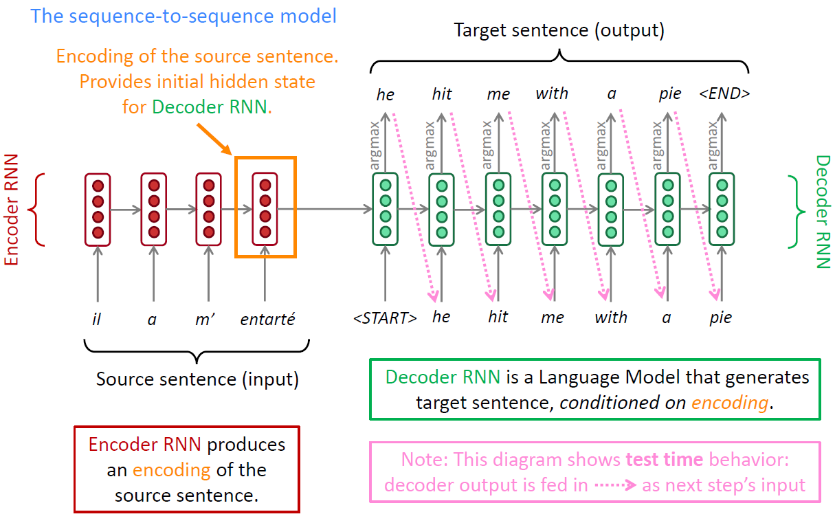
Neural Machine Translation, NMT

Sequence to sequence model:

seq2seq translation model

training a NMT model

NMT Training

The seq2seq model is an example of a Conditional Language Model. Decoder predicts the next word of the target sentence $\boldsymbol y$ conditioned on the source sentence $\boldsymbol x$ (encoder hidden state).

NMT directly calculates $P(\boldsymbol y|\boldsymbol x)$, NMT is generative model unlike SMT which is discriminative model:
$P(\boldsymbol y|\boldsymbol x)=\prod_{i=1}^TP(y_i|y_1,\cdots,y_{i-1},\boldsymbol x)$

Seq2Seq is optimized as a single system. Backpropagation operates “end-to-end”.

NMT Greedy Decoding

Greedy decoding that takes most probable word on each step of the decoder by taking argmax .

greedy decoding

prolems with greedy decoding

Beam Search Decoding

Find the optimal target sentence $\boldsymbol x$ by exhaustive search all possible sequences $\boldsymbol y$, $O(V^T)$ complexity, is far too expensive.

The core idea of beam search decoding is on each step of decoder, keep track of the $k$ most probable partial translations (which we call hypotheses), k is the beam size around 5 to 10 in practice. Beam search is not guaranteed to find optimal solution, but much more efficient.

Stopping Criterion

In greedy decoding, usually we decode until the model produces a token.

In beam search decoding, different hypotheses may produce token on different timesteps. When a hypothesis produces , that hypothesis is complete. Place is aside and continue exploring other hypotheses via beam search.

Usually we continue beam search until: we reach timestep $T$, or we have at least $n$ completed hypotheses ( $n$ and $T$ is some pre-defined cutoff.).

How to select top one with highest score?
$\text{score}(\boldsymbol y)=\log P_{\text{LM}}(\boldsymbol y|\boldsymbol x) = \sum_{i=1}^t\log P_{\text{LM}}(y_i|y_1,\cdots,y_{i-1},\boldsymbol x)$

Problem with this evaluation criteria: longer hypotheses have lower scores.

Fix: Normalize by length, use this to select top one instead:
$\frac{1}{t}\sum_{i=1}^t\log P_{\text{LM}}(y_i|y_1,\cdots,y_{i-1},\boldsymbol x)$

Advantages of NMT

NMT has many advantages compared to SMT: better performance, more fluent, better use of context, better use of phrase similarities, requires much less human engineering effort.

Challenges of NMT

Many difficulties remain: out-of-vocabulary words, domain mismatch between train and test data, maintaining context over longer text.

Attention

Using one encoding vector of the source sentence to decode/translate the target sentence, which needs to capture all information about the source sentence. This is information bottleneck.
Attention core idea: on each step of the decoder, use direct connection to the decoder to focus on a particular part of the source sequence.

Sequence-to-Sequence with Attention

Use attention distribution to take a weighted sum of the encoder hidden states, thus the decoder can decide (by self learning) which states to use to predict next word.
Attention provides some interpretability, we can see what the decoder was focusing on!

On each step $t$:

• Use the decoder hidden state $\boldsymbol h_t\in\R^h$ (query vector) with each encoder hidden state $\boldsymbol{\overline h_s}\in\R^h$ to compute the attention scores $\boldsymbol e_t\in\R^N$ (N timesteps).
  $e_t^s = \text{score}(\boldsymbol h_t, \boldsymbol{\overline h_s})= \begin{cases} \boldsymbol h_t^\top\boldsymbol{\overline h}_s &dot\\[.5ex] \boldsymbol h_t^\top\boldsymbol W_a\boldsymbol{\overline h}_s &general\\[.5ex] \boldsymbol v_a^\top\tanh(\boldsymbol W_a[\boldsymbol h_t;\boldsymbol{\overline h}_s]) &concat \end{cases}$

• Take softmax to get the attention distribution $\boldsymbol \alpha_t$.
  $\boldsymbol\alpha_t=\text{softmax}(\boldsymbol e_t)\in\R^N$

• Use $\boldsymbol\alpha_t$ to take a weighted sum of the overall encoder hidden states to compute the attention output $\boldsymbol c^t$ (global context vector), overall all the source states.
  $\boldsymbol c_t=\sum_{i=1}^N\alpha_t^i\boldsymbol{\overline h}_i \in \R^h$

• Employ a simple concatenation layer to combine the information from both vectors to produce an attentional hidden state.
  $\tilde{\boldsymbol h}_t=\tanh(\boldsymbol W_c[\boldsymbol c_t;\boldsymbol h_t])$

• The attention vector $\tilde{\boldsymbol h}_t$ is then fed through the softmax layer to produce the predictive distribution:
  $p(y_t|\boldsymbol y_{<t},\boldsymbol x) = \text{softmax}(\boldsymbol W_s\tilde{\boldsymbol h}_t)$

  
  

Implementation with Tensorflow

以下实现仅对于多分类任务，非NMT任务

def attention(inputs, inputs_size, atten_size):
    """
    atten_inputs:
    	(batch_size, max_time, hidden_size)
    expression:
    	u = tanh(w·h+b)
    	alpha = exp(u^t·v)/sum(exp(u^t·v))
    	s = sum(alpha·h)
    """
    hidden_size = int(inputs.shape[2])
    w = tf.Variable(tf.random_normal([hidden_size, atten_size]))
    b = tf.Variable(tf.random_normal([atten_size], stddev=0.1))
    v = tf.Variable(tf.random_normal([atten_size], stddev=0.1))
    
    # [batch_size, max_times, atten_size]
    u = tf.tanh(tf.matmul(inputs, w) + b)
    # [batch_size, max_times]
    uv = tf.linalg.matvec(u, v) / 2.0
    # set the alpha of padding symbol to zero by add negtive infinity number
    mask = tf.sequence_mask(inputs_size, max_len=TIME_STEPS, dtype=tf.float32)
    uv_mask = uv + tf.float32.min * (1- mask)
    alphas = tf.nn.softmax(uv_mask, axis=1)
    
    # [batch_size, max_times]
    # alphas = tf.exp(uv) * mask
    # alphas = alphas / tf.expand_dims(tf.reduce_sum(alphas, axis=1), -1)
    output = tf.reduce_sum(tf.multiply(inputs, tf.extend_dims(alphas, -1)), axis=1)
    
    return alphas, output

​