python List的特点
L=[i for i in range(10)] #对类型不做限定的list,同一个list中,每个元素的类型可以不一样,但是效率不高
L
[0, 1, 2, 3, 4, 5, 6, 7, 8, 9]
L[5]="Machine Learning"
L
[0, 1, 2, 3, 4, 'Machine Learning', 6, 7, 8, 9]
import array
arr = array.array('i',[i for i in range(10)]) #只能存储一种类型数据、效率比较高,没有将数据看做是向量或者矩阵,没有配备相关的运算
arr[5]
5
arr[5]="Machine Learning"
---------------------------------------------------------------------------

TypeError                                 Traceback (most recent call last)

<ipython-input-51-614ba609ccbc> in <module>
----> 1 arr[5]="Machine Learning"


TypeError: an integer is required (got type str)
numpy.array
nparr = np.array([i for i in range(10)])
nparr
array([0, 1, 2, 3, 4, 5, 6, 7, 8, 9])
nparr[5] = 100
nparr
array([ 0, 1, 2, 3, 4, 100, 6, 7, 8, 9])
nparr[5]='Machine Learning'
---------------------------------------------------------------------------

ValueError                                Traceback (most recent call last)

<ipython-input-54-b468797a806a> in <module>
----> 1 nparr[5]='Machine Learning'


ValueError: invalid literal for int() with base 10: 'Machine Learning'
#numpy array 与 list array用法相似,也只能存储一种类型数据
nparr.dtype #默认是int64
dtype('int32')
nparr[5]=0.5
nparr
array([0, 1, 2, 3, 4, 0, 6, 7, 8, 9])
nparr.dtype
dtype('int32')
nparr[3]=3.14
nparr
array([0, 1, 2, 3, 4, 0, 6, 7, 8, 9])
nparr2 = np.array([1,2,3.0])
nparr2.dtype
dtype('float64')
nparr2
array([1., 2., 3.])
其他创建numpy.array的方法
np.zeros(10)
array([0., 0., 0., 0., 0., 0., 0., 0., 0., 0.])
np.zeros(10).dtype
dtype('float64')
np.zeros(10,dtype=int)
array([0, 0, 0, 0, 0, 0, 0, 0, 0, 0])
np.zeros((3,5))
array([[0., 0., 0., 0., 0.],
       [0., 0., 0., 0., 0.],
       [0., 0., 0., 0., 0.]])
np.zeros(shape=(3,5),dtype=int)
array([[0, 0, 0, 0, 0],
       [0, 0, 0, 0, 0],
       [0, 0, 0, 0, 0]])
np.ones(10)
array([1., 1., 1., 1., 1., 1., 1., 1., 1., 1.])
np.ones((3,5))
array([[1., 1., 1., 1., 1.],
       [1., 1., 1., 1., 1.],
       [1., 1., 1., 1., 1.]])
np.full(shape=(3,5),fill_value=666)
array([[666, 666, 666, 666, 666],
       [666, 666, 666, 666, 666],
       [666, 666, 666, 666, 666]])
np.full(shape=(3,5),fill_value=666.0)
array([[666., 666., 666., 666., 666.],
       [666., 666., 666., 666., 666.],
       [666., 666., 666., 666., 666.]])
arange
[i for i in range(0,20,2)]
[0, 2, 4, 6, 8, 10, 12, 14, 16, 18]
np.arange(0,20,2)
array([ 0, 2, 4, 6, 8, 10, 12, 14, 16, 18])
[i for i in range(0,1,0.2)]
---------------------------------------------------------------------------

TypeError                                 Traceback (most recent call last)

<ipython-input-14-be9c9326671d> in <module>
----> 1 [i for i in range(0,1,0.2)]


TypeError: 'float' object cannot be interpreted as an integer
np.arange(0,1,0.2)
array([0. , 0.2, 0.4, 0.6, 0.8])
np.arange(0,10)
array([0, 1, 2, 3, 4, 5, 6, 7, 8, 9])
np.arange(10)
array([0, 1, 2, 3, 4, 5, 6, 7, 8, 9])
linspace
np.linspace(0,20,10) #等长的截出十个点
array([ 0.        ,  2.22222222,  4.44444444,  6.66666667,  8.88888889,
       11.11111111, 13.33333333, 15.55555556, 17.77777778, 20.        ])
np.linspace(0,20,11)
array([ 0., 2., 4., 6., 8., 10., 12., 14., 16., 18., 20.])
random
import numpy as np
np.random.randint(0,10)
5
np.random.randint(0,10,10)
array([5, 3, 1, 6, 2, 8, 0, 0, 9, 9])
np.random.randint(0,1,5)
array([0, 0, 0, 0, 0])
np.random.randint(4,8,size=10)
array([6, 6, 4, 7, 6, 6, 4, 7, 6, 4])
np.random.randint(4,8,size=(3,5))
array([[6, 5, 4, 4, 4],
       [4, 6, 4, 7, 6],
       [6, 5, 4, 4, 5]])
np.random.seed(666)#随机种子
np.random.randint(4,8,size=(3,5))
array([[4, 6, 5, 6, 6],
       [6, 5, 6, 4, 5],
       [7, 6, 7, 4, 7]])
np.random.seed(666)#随机种子
np.random.randint(4,8,size=(3,5))
array([[4, 6, 5, 6, 6],
       [6, 5, 6, 4, 5],
       [7, 6, 7, 4, 7]])
np.random.random() #生成0,1之间的随机浮点数
0.2811684913927954
np.random.random((3,5))
array([[0.46284169, 0.23340091, 0.76706421, 0.81995656, 0.39747625],
       [0.31644109, 0.15551206, 0.73460987, 0.73159555, 0.8578588 ],
       [0.76741234, 0.95323137, 0.29097383, 0.84778197, 0.3497619 ]])
np.random.normal(10,100) #符合均值为10,方差为100正态分布的随机数
-11.326813235544162
np.random.normal(0,1,(3,5))
array([[ 0.18305429,  0.34543496, -0.8131543 ,  1.06325382,  0.25866385],
       [ 0.47285107,  1.0319698 , -0.16045655,  0.00592353, -0.53452616],
       [ 1.15170083, -1.34498108, -0.36119241, -1.15146822,  0.49224775]])
help(np.random.normal)
Help on built-in function normal:

normal(...) method of mtrand.RandomState instance
    normal(loc=0.0, scale=1.0, size=None)

    Draw random samples from a normal (Gaussian) distribution.

    The probability density function of the normal distribution, first
    derived by De Moivre and 200 years later by both Gauss and Laplace
    independently [2]_, is often called the bell curve because of
    its characteristic shape (see the example below).

    The normal distributions occurs often in nature.  For example, it
    describes the commonly occurring distribution of samples influenced
    by a large number of tiny, random disturbances, each with its own
    unique distribution [2]_.

    Parameters
    ----------
    loc : float or array_like of floats
        Mean ("centre") of the distribution.
    scale : float or array_like of floats
        Standard deviation (spread or "width") of the distribution.
    size : int or tuple of ints, optional
        Output shape.  If the given shape is, e.g., ``(m, n, k)``, then
        ``m * n * k`` samples are drawn.  If size is ``None`` (default),
        a single value is returned if ``loc`` and ``scale`` are both scalars.
        Otherwise, ``np.broadcast(loc, scale).size`` samples are drawn.

    Returns
    -------
    out : ndarray or scalar
        Drawn samples from the parameterized normal distribution.

    See Also
    --------
    scipy.stats.norm : probability density function, distribution or
        cumulative density function, etc.

    Notes
    -----
    The probability density for the Gaussian distribution is

    .. math:: p(x) = \frac{1}{\sqrt{ 2 \pi \sigma^2 }}
                     e^{ - \frac{ (x - \mu)^2 } {2 \sigma^2} },

    where :math:`\mu` is the mean and :math:`\sigma` the standard
    deviation. The square of the standard deviation, :math:`\sigma^2`,
    is called the variance.

    The function has its peak at the mean, and its "spread" increases with
    the standard deviation (the function reaches 0.607 times its maximum at
    :math:`x + \sigma` and :math:`x - \sigma` [2]_).  This implies that
    `numpy.random.normal` is more likely to return samples lying close to
    the mean, rather than those far away.

    References
    ----------
    .. [1] Wikipedia, "Normal distribution",
           https://en.wikipedia.org/wiki/Normal_distribution
    .. [2] P. R. Peebles Jr., "Central Limit Theorem" in "Probability,
           Random Variables and Random Signal Principles", 4th ed., 2001,
           pp. 51, 51, 125.

    Examples
    --------
    Draw samples from the distribution:

    >>> mu, sigma = 0, 0.1 # mean and standard deviation
    >>> s = np.random.normal(mu, sigma, 1000)

    Verify the mean and the variance:

    >>> abs(mu - np.mean(s)) < 0.01
    True

    >>> abs(sigma - np.std(s, ddof=1)) < 0.01
    True

    Display the histogram of the samples, along with
    the probability density function:

    >>> import matplotlib.pyplot as plt
    >>> count, bins, ignored = plt.hist(s, 30, density=True)
    >>> plt.plot(bins, 1/(sigma * np.sqrt(2 * np.pi)) *
    ...                np.exp( - (bins - mu)**2 / (2 * sigma**2) ),
    ...          linewidth=2, color='r')
    >>> plt.show()
np.__version__
'1.16.2'
Numpy array 的基本操作
import numpy as np
x=np.arange(10)
x
array([0, 1, 2, 3, 4, 5, 6, 7, 8, 9])
X=np.arange(15).reshape(3,5)
X
array([[ 0,  1,  2,  3,  4],
       [ 5,  6,  7,  8,  9],
       [10, 11, 12, 13, 14]])
基本属性
x.ndim #查看数组的维数
1
X.ndim
2
x.shape#查看数组的维度
(10,)
X.shape
(3, 5)
x.size#查看数组的元素个数
10
X.size
15
numpy.array 的数据访问
x
array([0, 1, 2, 3, 4, 5, 6, 7, 8, 9])
x[0]
0
x[-1]
9
X[0][0] #不建议这么写
0
X[2,2] #建议这么访问,即使是访问1个元素,也使用这种方式
12
x[0:5]#切片
array([0, 1, 2, 3, 4])
x[:5]
array([0, 1, 2, 3, 4])
x[5:]
array([5, 6, 7, 8, 9])
x[::2]
array([0, 2, 4, 6, 8])
x[::-1]
array([9, 8, 7, 6, 5, 4, 3, 2, 1, 0])
X
array([[ 0,  1,  2,  3,  4],
       [ 5,  6,  7,  8,  9],
       [10, 11, 12, 13, 14]])
X[:2,:3]#依次为行切片、列切片
array([[0, 1, 2],
       [5, 6, 7]])
X[:2][:3] #使用两个中括号访问会出错
array([[0, 1, 2, 3, 4],
       [5, 6, 7, 8, 9]])
X[:2]
array([[0, 1, 2, 3, 4],
       [5, 6, 7, 8, 9]])
X[:2,::2]
array([[0, 2, 4],
       [5, 7, 9]])
X[::-1,::-1]
array([[14, 13, 12, 11, 10],
       [ 9,  8,  7,  6,  5],
       [ 4,  3,  2,  1,  0]])
X[0]
array([0, 1, 2, 3, 4])
X[0,:]#只取一行
array([0, 1, 2, 3, 4])
X[0,:].ndim
1
X[:,0]#只取一列
array([ 0, 5, 10])
X[:,0].ndim
1
subX=X[:2,:3] #子矩阵
subX
array([[0, 1, 2],
       [5, 6, 7]])
subX[0,0]=100
subX
array([[100,   1,   2],
       [  5,   6,   7]])
X#修改子矩阵,原矩阵也会被影响
array([[100,   1,   2,   3,   4],
       [  5,   6,   7,   8,   9],
       [ 10,  11,  12,  13,  14]])
X[0,0]=0
X
array([[ 0,  1,  2,  3,  4],
       [ 5,  6,  7,  8,  9],
       [10, 11, 12, 13, 14]])
subX#同理,修改原矩阵,子矩阵也会被影响
array([[0, 1, 2],
       [5, 6, 7]])
subX=X[:2,:3].copy()#这种方式获得的子矩阵就与原矩阵脱离了关系,改变后,相互不影响
subX
array([[0, 1, 2],
       [5, 6, 7]])
subX[0,0]=100
subX
array([[100,   1,   2],
       [  5,   6,   7]])
X
array([[ 0,  1,  2,  3,  4],
       [ 5,  6,  7,  8,  9],
       [10, 11, 12, 13, 14]])
Reshape
#数组中的数字不需要改变,需要改变数组中的维度
x.reshape(2,5)
array([[0, 1, 2, 3, 4],
       [5, 6, 7, 8, 9]])
x
array([0, 1, 2, 3, 4, 5, 6, 7, 8, 9])
A=x.reshape(2,5) #改变成两行五列
A
array([[0, 1, 2, 3, 4],
       [5, 6, 7, 8, 9]])
B=x.reshape(1,10) #改变成一行十列,注意:是一个二维数组
B
array([[0, 1, 2, 3, 4, 5, 6, 7, 8, 9]])
B.ndim #有两个维度
2
B.shape #有两个维度:1行,10列
(1, 10)
x.shape
(10,)
x.reshape(10,-1)#指定第一个维度的数据,另外一个维度的依靠计算机的智能计算
array([[0],
       [1],
       [2],
       [3],
       [4],
       [5],
       [6],
       [7],
       [8],
       [9]])
x.reshape(2,-1)
array([[0, 1, 2, 3, 4],
       [5, 6, 7, 8, 9]])
x.reshape(3,-1)
---------------------------------------------------------------------------

ValueError                                Traceback (most recent call last)

<ipython-input-60-27fb2acd3ab6> in <module>
----> 1 x.reshape(3,-1)


ValueError: cannot reshape array of size 10 into shape (3,newaxis)
合并
import numpy as np
x = np.array([1,2,3])
y=np.array([3,2,1])
x
array([1, 2, 3])
y
array([3, 2, 1])
np.concatenate([x,y])#x、y合并
array([1, 2, 3, 3, 2, 1])
z=np.array([666,666,666])#一维向量
np.concatenate([x,y,z])
array([ 1, 2, 3, 3, 2, 1, 666, 666, 666])
A = np.array([[1,2,3],[4,5,6]])#二维矩阵
np.concatenate([A,A])#默认axis=0,连接结果是一个新的矩阵
array([[1, 2, 3],
       [4, 5, 6],
       [1, 2, 3],
       [4, 5, 6]])
np.concatenate([A,A],axis=1) #axis=1表示沿着列的方向进行拼接
array([[1, 2, 3, 1, 2, 3],
       [4, 5, 6, 4, 5, 6]])
np.concatenate([A,z]) #只能处理维数一样的数据
---------------------------------------------------------------------------

ValueError                                Traceback (most recent call last)

<ipython-input-13-abdc54b54f98> in <module>
----> 1 np.concatenate([A,z])


ValueError: all the input arrays must have same number of dimensions
np.concatenate([A,z.reshape(1,-1)]) #将z转换成二维矩阵后,可合并连接
array([[  1,   2,   3],
       [  4,   5,   6],
       [666, 666, 666]])
A#连接结果是一个新的矩阵,此时A依然是原来的数据
array([[1, 2, 3],
       [4, 5, 6]])
np.vstack([A,z])#在垂直的方向,进行数据的堆叠。这种方式容错性更好,即使维度不同,也可以只能的进行合并拼接
array([[  1,   2,   3],
       [  4,   5,   6],
       [666, 666, 666]])
B = np.full((2,2),100)
B
array([[100, 100],
       [100, 100]])
np.hstack([A,B])#在水平方向,进行数据的堆叠。
array([[  1,   2,   3, 100, 100],
       [  4,   5,   6, 100, 100]])
np.hstack([A,z]) #在水平方向,无法堆叠
---------------------------------------------------------------------------

ValueError                                Traceback (most recent call last)

<ipython-input-23-c82760796347> in <module>
----> 1 np.hstack([A,z]) #在水平方向,无法堆叠


D:\Anaconda3\lib\site-packages\numpy\core\shape_base.py in hstack(tup)
    338         return _nx.concatenate(arrs, 0)
    339     else:
--> 340         return _nx.concatenate(arrs, 1)
    341
    342


ValueError: all the input arrays must have same number of dimensions
分割操作
x = np.arange(10)
x
array([0, 1, 2, 3, 4, 5, 6, 7, 8, 9])
x1,x2,x3 = np.split(x,[3,7]) #第一个参数是待分割数组,第二个参数是分割点,此处有两个分割点
x1
array([0, 1, 2])
x2
array([3, 4, 5, 6])
x3
array([7, 8, 9])
x1,x2=np.split(x,[5])
x1
array([0, 1, 2, 3, 4])
x2
array([5, 6, 7, 8, 9])
A = np.arange(16).reshape((4,4))
A
array([[ 0,  1,  2,  3],
       [ 4,  5,  6,  7],
       [ 8,  9, 10, 11],
       [12, 13, 14, 15]])
A1,A2=np.split(A,[2]) #在行的维度上分割
A1
array([[0, 1, 2, 3],
       [4, 5, 6, 7]])
A2
array([[ 8,  9, 10, 11],
       [12, 13, 14, 15]])
A1,A2=np.split(A,[2],axis=1) #在列的维度上分割
A1
array([[ 0,  1],
       [ 4,  5],
       [ 8,  9],
       [12, 13]])
A2
array([[ 2,  3],
       [ 6,  7],
       [10, 11],
       [14, 15]])
upper,lower=np.vsplit(A,[2])
upper
array([[0, 1, 2, 3],
       [4, 5, 6, 7]])
lower
array([[ 8,  9, 10, 11],
       [12, 13, 14, 15]])
left,right=np.hsplit(A,[2]) #水平方向分割
left
array([[ 0,  1],
       [ 4,  5],
       [ 8,  9],
       [12, 13]])
right
array([[ 2,  3],
       [ 6,  7],
       [10, 11],
       [14, 15]])
data = np.arange(16).reshape((4,4))
data
array([[ 0,  1,  2,  3],
       [ 4,  5,  6,  7],
       [ 8,  9, 10, 11],
       [12, 13, 14, 15]])
x,y = np.hsplit(data,[-1])
x
array([[ 0,  1,  2],
       [ 4,  5,  6],
       [ 8,  9, 10],
       [12, 13, 14]])
y
array([[ 3],
       [ 7],
       [11],
       [15]])
y[:,0]
array([ 3, 7, 11, 15])
numpy.array中的运算
给定一个向量,让向量中每一个数乘以2
a=(0,1,2)
a*2=(0,2,4)
n=10
L=[i for i in range(n)]
2*L #将两个相同的列表首尾相连,并不是我们想要的效果(列表中的每个元素都乘2)
[0, 1, 2, 3, 4, 5, 6, 7, 8, 9, 0, 1, 2, 3, 4, 5, 6, 7, 8, 9]
A=[]
for e in L:
    A.append(2*e)
A
[0, 2, 4, 6, 8, 10, 12, 14, 16, 18]
n = 1000000
L = [i for i in range(n)]
%%time
A = []
for e in L:
    A.append(2*e)  #测试时间效率
Wall time: 132 ms
%%time
A = [2*e for e in L] #列表生成式的
Wall time: 72.9 ms
import numpy as np
L = np.arange(n)
%%time
A = np.array(2*e for e in L)  #可以发现运行速度很快,效率极高,和python的list不是一个数量级
Wall time: 0 ns
%%time
A = 2*L
Wall time: 1.99 ms
A
[0, 2, 4, 6, 8, 10, 12, 14, 16, 18]
L
array([ 0, 1, 2, ..., 999997, 999998, 999999])
%%time
A = 2*L
Wall time: 2.48 ms
2*L#可以实现效果(列表中每个元素都乘2)
array([ 0, 2, 4, ..., 1999994, 1999996, 1999998])
Universal Functions
X = np.arange(1,16).reshape((3,5))
X
array([[ 1,  2,  3,  4,  5],
       [ 6,  7,  8,  9, 10],
       [11, 12, 13, 14, 15]])
X+1
array([[ 2,  3,  4,  5,  6],
       [ 7,  8,  9, 10, 11],
       [12, 13, 14, 15, 16]])
X-1
array([[ 0,  1,  2,  3,  4],
       [ 5,  6,  7,  8,  9],
       [10, 11, 12, 13, 14]])
X*2
array([[ 2,  4,  6,  8, 10],
       [12, 14, 16, 18, 20],
       [22, 24, 26, 28, 30]])
X/2 #浮点数除法
array([[0.5, 1. , 1.5, 2. , 2.5],
       [3. , 3.5, 4. , 4.5, 5. ],
       [5.5, 6. , 6.5, 7. , 7.5]])
X//2 #整除
array([[0, 1, 1, 2, 2],
       [3, 3, 4, 4, 5],
       [5, 6, 6, 7, 7]], dtype=int32)
X**2 #幂运算
array([[  1,   4,   9,  16,  25],
       [ 36,  49,  64,  81, 100],
       [121, 144, 169, 196, 225]], dtype=int32)
X%2 #取余运算
array([[1, 0, 1, 0, 1],
       [0, 1, 0, 1, 0],
       [1, 0, 1, 0, 1]], dtype=int32)
1/X #取倒数
array([[1.        , 0.5       , 0.33333333, 0.25      , 0.2       ],
       [0.16666667, 0.14285714, 0.125     , 0.11111111, 0.1       ],
       [0.09090909, 0.08333333, 0.07692308, 0.07142857, 0.06666667]])
np.abs(X) #绝对值
array([[ 1,  2,  3,  4,  5],
       [ 6,  7,  8,  9, 10],
       [11, 12, 13, 14, 15]])
np.sin(X) #正弦函数
array([[ 0.84147098,  0.90929743,  0.14112001, -0.7568025 , -0.95892427],
       [-0.2794155 ,  0.6569866 ,  0.98935825,  0.41211849, -0.54402111],
       [-0.99999021, -0.53657292,  0.42016704,  0.99060736,  0.65028784]])
np.cos(X) #余弦函数
array([[ 0.54030231, -0.41614684, -0.9899925 , -0.65364362,  0.28366219],
       [ 0.96017029,  0.75390225, -0.14550003, -0.91113026, -0.83907153],
       [ 0.0044257 ,  0.84385396,  0.90744678,  0.13673722, -0.75968791]])
np.tan(X) #正切函数
array([[ 1.55740772e+00, -2.18503986e+00, -1.42546543e-01,
         1.15782128e+00, -3.38051501e+00],
       [-2.91006191e-01,  8.71447983e-01, -6.79971146e+00,
        -4.52315659e-01,  6.48360827e-01],
       [-2.25950846e+02, -6.35859929e-01,  4.63021133e-01,
         7.24460662e+00, -8.55993401e-01]])
np.exp(X)
array([[2.71828183e+00, 7.38905610e+00, 2.00855369e+01, 5.45981500e+01,
        1.48413159e+02],
       [4.03428793e+02, 1.09663316e+03, 2.98095799e+03, 8.10308393e+03,
        2.20264658e+04],
       [5.98741417e+04, 1.62754791e+05, 4.42413392e+05, 1.20260428e+06,
        3.26901737e+06]])
np.power(3,x)#3的x次方
array([[       3,        9,       27,       81,      243],
       [     729,     2187,     6561,    19683,    59049],
       [  177147,   531441,  1594323,  4782969, 14348907]], dtype=int32)
3**X #与np.power(3,x)结果一致
array([[       3,        9,       27,       81,      243],
       [     729,     2187,     6561,    19683,    59049],
       [  177147,   531441,  1594323,  4782969, 14348907]], dtype=int32)
np.log(X)
array([[0.        , 0.69314718, 1.09861229, 1.38629436, 1.60943791],
       [1.79175947, 1.94591015, 2.07944154, 2.19722458, 2.30258509],
       [2.39789527, 2.48490665, 2.56494936, 2.63905733, 2.7080502 ]])
np.log2(X)
array([[0.        , 1.        , 1.5849625 , 2.        , 2.32192809],
       [2.5849625 , 2.80735492, 3.        , 3.169925  , 3.32192809],
       [3.45943162, 3.5849625 , 3.70043972, 3.80735492, 3.9068906 ]])
np.log10(X)
array([[0.        , 0.30103   , 0.47712125, 0.60205999, 0.69897   ],
       [0.77815125, 0.84509804, 0.90308999, 0.95424251, 1.        ],
       [1.04139269, 1.07918125, 1.11394335, 1.14612804, 1.17609126]])
矩阵运算
A = np.arange(4).reshape(2,2)
A
array([[0, 1],
       [2, 3]])
B = np.full((2,2),10)
B
array([[10, 10],
       [10, 10]])
A+B
array([[10, 11],
       [12, 13]])
A-B
array([[-10,  -9],
       [ -8,  -7]])
A*B #在numpy中,所有矩阵做运算,都是矩阵中对应元素做计算
array([[ 0, 10],
       [20, 30]])
A/B
array([[0. , 0.1],
       [0.2, 0.3]])
A.dot(B)#矩阵的乘法
array([[10, 10],
       [50, 50]])
A.T #矩阵的转置
array([[0, 2],
       [1, 3]])
C = np.full((3,3),666)
A+C #2×2矩阵和3×3矩阵之间不能做加法
---------------------------------------------------------------------------

ValueError                                Traceback (most recent call last)

<ipython-input-51-ad27a378f233> in <module>
----> 1 A+C  #2×2矩阵和3×3矩阵之间不能做加法


ValueError: operands could not be broadcast together with shapes (2,2) (3,3)
A.dot(C) #也不能做乘法
---------------------------------------------------------------------------

ValueError                                Traceback (most recent call last)

<ipython-input-52-d4c5cc1c57d3> in <module>
----> 1 A.dot(C) #也不能做乘法


ValueError: shapes (2,2) and (3,3) not aligned: 2 (dim 1) != 3 (dim 0)
向量和矩阵的运算
V = np.array([1,2])
A
array([[0, 1],
       [2, 3]])
V+A
array([[1, 3],
       [3, 5]])
np.vstack([V]*A.shape[0])
array([[1, 2],
       [1, 2]])
np.vstack([V]*A.shape[0]) +A
array([[1, 3],
       [3, 5]])
np.tile(V,(2,1))# 在行向量上堆叠2次,在列向量上堆叠1次
array([[1, 2],
       [1, 2]])
np.tile(V,(2,1))+A
array([[1, 3],
       [3, 5]])
V
array([1, 2])
A
array([[0, 1],
       [2, 3]])
V*A
array([[0, 2],
       [2, 6]])
V.dot(A) #满足矩阵乘法的用法
array([4, 7])
矩阵的逆
A
array([[0, 1],
       [2, 3]])
invA=np.linalg.inv(A) #A的逆矩阵
A.dot(invA) #原矩阵乘以逆矩阵等于单位矩阵,只有方阵才有逆矩阵
array([[1., 0.],
       [0., 1.]])
invA.dot(A)
array([[1., 0.],
       [0., 1.]])
X = np.arange(16).reshape((2,8))
X
array([[ 0,  1,  2,  3,  4,  5,  6,  7],
       [ 8,  9, 10, 11, 12, 13, 14, 15]])
np.linalg.inv(x) #对于这个2x8的矩阵,无法求逆矩阵
---------------------------------------------------------------------------

LinAlgError                               Traceback (most recent call last)

<ipython-input-76-8b65a3a47f10> in <module>
----> 1 np.linalg.inv(x) #对于这个2x8的矩阵,无法求逆矩阵


D:\Anaconda3\lib\site-packages\numpy\linalg\linalg.py in inv(a)
    544     a, wrap = _makearray(a)
    545     _assertRankAtLeast2(a)
--> 546     _assertNdSquareness(a)
    547     t, result_t = _commonType(a)
    548


D:\Anaconda3\lib\site-packages\numpy\linalg\linalg.py in _assertNdSquareness(*arrays)
    211         m, n = a.shape[-2:]
    212         if m != n:
--> 213             raise LinAlgError('Last 2 dimensions of the array must be square')
    214
    215 def _assertFinite(*arrays):


LinAlgError: Last 2 dimensions of the array must be square
pinvX = np.linalg.pinv(X)#求伪逆矩阵
X.dot(pinvX)
array([[ 1.00000000e+00, -2.49800181e-16],
       [ 0.00000000e+00,  1.00000000e+00]])
[array([1, 2])]
array([[1, 2],
       [1, 2]])
[array([1, 2]), array([1, 2])]
聚合操作
import numpy as np
L = np.random.random(100)
L
array([0.1228489 , 0.10128162, 0.73890636, 0.81042729, 0.19496766,
       0.80428713, 0.86513596, 0.14653162, 0.92144986, 0.67895328,
       0.75577749, 0.23335295, 0.58914832, 0.90760158, 0.87885077,
       0.83456836, 0.30622795, 0.48560068, 0.80300485, 0.0178615 ,
       0.22154929, 0.85884983, 0.10643329, 0.60619614, 0.53585217,
       0.28598115, 0.53559168, 0.95226976, 0.71352252, 0.39687969,
       0.86367034, 0.46117165, 0.41006472, 0.29836383, 0.97847759,
       0.58180827, 0.34688957, 0.53062455, 0.17021749, 0.03279539,
       0.78377669, 0.65252611, 0.3765404 , 0.16559353, 0.89126029,
       0.64086652, 0.82790449, 0.52387458, 0.01787634, 0.56585925,
       0.24946476, 0.81287152, 0.33010826, 0.07630455, 0.63620404,
       0.20490412, 0.02943005, 0.4076763 , 0.42475491, 0.70963187,
       0.55176048, 0.94883838, 0.33103014, 0.99172951, 0.82672215,
       0.89685283, 0.14469067, 0.15907508, 0.36760791, 0.51101058,
       0.14605049, 0.97852068, 0.29914652, 0.89837895, 0.18190285,
       0.05308824, 0.77889743, 0.76967326, 0.38211872, 0.48344965,
       0.3377394 , 0.1575669 , 0.00176385, 0.93624582, 0.49509178,
       0.63326002, 0.97418133, 0.79167643, 0.07677647, 0.03987844,
       0.36851419, 0.37962724, 0.1225014 , 0.27308183, 0.14032391,
       0.44501452, 0.29975825, 0.45586269, 0.04763424, 0.25704284])
sum(L) #python中list求和
48.34550769673254
np.sum(L) #numpy求和得方式,效率更高
48.34550769673254
big_array = np.random.rand(10000)
%timeit sum(big_array)
%timeit np.sum(big_array)
720 µs ± 12.6 µs per loop (mean ± std. dev. of 7 runs, 1000 loops each)
5.65 µs ± 132 ns per loop (mean ± std. dev. of 7 runs, 100000 loops each)
np.min(big_array) #求一组数的最小值
5.061695669594801e-05
np.max(big_array) #求一组数的最大值
0.9998519913880158
big_array.min()#求一组数的最小值的另一种方式
5.061695669594801e-05
big_array.max()#求一组数的最大值的另一种方式
0.9998519913880158
big_array.sum()#求一组数和的另一种方式
4961.205582580736
X = np.arange(16).reshape(4,-1)
X
array([[ 0,  1,  2,  3],
       [ 4,  5,  6,  7],
       [ 8,  9, 10, 11],
       [12, 13, 14, 15]])
np.sum(X)
120
np.sum(X,axis=0) #每列相加,沿着行的方向进行相加
array([24, 28, 32, 36])
np.sum(X,axis=1) #沿着列的方向进行相加
array([ 6, 22, 38, 54])
np.prod(X) #各元素相乘
0
np.prod(X+1) #每个元素都加1,再相乘
2004189184
v = np.array([1,1,2,2,10])
np.mean(v) #求平均值
3.2
np.median(v) #求中位数
2.0
np.percentile(big_array,q=50) #求百分位数
0.49504621587472625
for percent in [0,25,50,75,100]:
    print(np.percentile(big_array,q=percent))
5.061695669594801e-05
0.2453212464370438
0.49504621587472625
0.7451722008762793
0.9998519913880158
np.var(big_array) #求方差
0.08365793041233283
np.std(big_array) #标准差
0.28923680680773123
x = np.random.normal(0,1,size=10000000)
np.mean(x)
0.00011898517652053636
np.std(x)
1.000276806205529
索引
np.min(x)
-5.408035633629394
np.argmin(x) #最小值的索引位置
8777314
x[8777314] #根据索引值获得最小值
-5.408035633629394
np.argmax(x)
5885565
x[5885565]
5.3195730493141875
np.max(x)
5.3195730493141875
排序和使用索引
x = np.arange(16)
x
array([ 0, 1, 2, 3, 4, 5, 6, 7, 8, 9, 10, 11, 12, 13, 14, 15])
np.random.shuffle(x) #乱序处理
x
array([ 5, 7, 15, 9, 3, 10, 0, 4, 8, 2, 11, 1, 6, 14, 12, 13])
np.sort(x) #排序
array([ 0, 1, 2, 3, 4, 5, 6, 7, 8, 9, 10, 11, 12, 13, 14, 15])
x #x还是乱序
array([ 5, 7, 15, 9, 3, 10, 0, 4, 8, 2, 11, 1, 6, 14, 12, 13])
x.sort()
x   #x不是乱序
array([ 0, 1, 2, 3, 4, 5, 6, 7, 8, 9, 10, 11, 12, 13, 14, 15])
X = np.random.randint(10,size=(4,4))
X
array([[5, 2, 5, 0],
       [8, 5, 8, 2],
       [3, 9, 3, 2],
       [6, 3, 9, 4]])
np.sort(X)
array([[0, 2, 5, 5],
       [2, 5, 8, 8],
       [2, 3, 3, 9],
       [3, 4, 6, 9]])
np.sort(X,axis=1)
array([[0, 2, 5, 5],
       [2, 5, 8, 8],
       [2, 3, 3, 9],
       [3, 4, 6, 9]])
np.sort(X,axis=0)
array([[3, 2, 3, 0],
       [5, 3, 5, 2],
       [6, 5, 8, 2],
       [8, 9, 9, 4]])
x
array([ 0, 1, 2, 3, 4, 5, 6, 7, 8, 9, 10, 11, 12, 13, 14, 15])
np.random.shuffle(x)
x
array([ 4, 14, 3, 5, 2, 1, 7, 12, 15, 8, 0, 9, 10, 13, 11, 6])
np.argsort(x) #存放的是元素的索引,按照原数组索引有序排序
array([10,  5,  4,  2,  0,  3, 15,  6,  9, 11, 12, 14,  7, 13,  1,  8],
      dtype=int64)
np.partition(x,3) #和数字3进行比较,比3大的数据排在3前面,比3小的数据排在3后面
array([ 0, 1, 2, 3, 4, 5, 6, 14, 15, 8, 7, 9, 10, 13, 11, 12])
np.argpartition(x,3)#返回的值是索引
array([10,  5,  4,  2,  0,  3, 15,  1,  8,  9,  6, 11, 12, 13, 14,  7],
      dtype=int64)
X
array([[5, 2, 5, 0],
       [8, 5, 8, 2],
       [3, 9, 3, 2],
       [6, 3, 9, 4]])
np.argsort(X,axis=1)
array([[3, 1, 0, 2],
       [3, 1, 0, 2],
       [3, 0, 2, 1],
       [1, 3, 0, 2]], dtype=int64)
np.argsort(X,axis=0)
array([[2, 0, 2, 0],
       [0, 3, 0, 1],
       [3, 1, 1, 2],
       [1, 2, 3, 3]], dtype=int64)
np.argpartition(X,2,axis=1)
array([[3, 1, 2, 0],
       [3, 1, 2, 0],
       [3, 2, 0, 1],
       [1, 3, 0, 2]], dtype=int64)
np.argpartition(X,2,axis=0)
array([[2, 0, 2, 0],
       [0, 3, 0, 1],
       [3, 1, 1, 2],
       [1, 2, 3, 3]], dtype=int64)
Fancy Indexing
import numpy as np

x = np.arange(16)
x
array([ 0, 1, 2, 3, 4, 5, 6, 7, 8, 9, 10, 11, 12, 13, 14, 15])
x[3] #索引值
3
x[3:9:2] #索引区间,切片
array([3, 5, 7])
[x[3],x[5],x[8]] #访问没有规律的索引区间
[3, 5, 8]
ind = [3,5,8] #将索引存到列表中
x[ind]
array([3, 5, 8])
ind = np.array([[0,2],
               [1,3]])
x[ind]
array([[0, 2],
       [1, 3]])
X = x.reshape(4,-1)
X
array([[ 0,  1,  2,  3],
       [ 4,  5,  6,  7],
       [ 8,  9, 10, 11],
       [12, 13, 14, 15]])
row = np.array([0,1,2])
col = np.array([1,2,3])
X[row,col]
array([ 1, 6, 11])
X[0,col]
array([1, 2, 3])
X[:2,col]
array([[1, 2, 3],
       [5, 6, 7]])
col = [True,False,True,True]
X[1:3,col]
array([[ 4,  6,  7],
       [ 8, 10, 11]])
numpy.array的比较
x
array([ 0, 1, 2, 3, 4, 5, 6, 7, 8, 9, 10, 11, 12, 13, 14, 15])
x<3
array([ True,  True,  True, False, False, False, False, False, False,
       False, False, False, False, False, False, False])
x>3
array([False, False, False, False,  True,  True,  True,  True,  True,
        True,  True,  True,  True,  True,  True,  True])
x<=3
array([ True,  True,  True,  True, False, False, False, False, False,
       False, False, False, False, False, False, False])
x>=3
array([False, False, False,  True,  True,  True,  True,  True,  True,
        True,  True,  True,  True,  True,  True,  True])
x==3
array([False, False, False,  True, False, False, False, False, False,
       False, False, False, False, False, False, False])
x!=3
array([ True,  True,  True, False,  True,  True,  True,  True,  True,
        True,  True,  True,  True,  True,  True,  True])
2*x == 24-4*x
array([False, False, False, False,  True, False, False, False, False,
       False, False, False, False, False, False, False])
X
array([[ 0,  1,  2,  3],
       [ 4,  5,  6,  7],
       [ 8,  9, 10, 11],
       [12, 13, 14, 15]])
X<6
array([[ True,  True,  True,  True],
       [ True,  True, False, False],
       [False, False, False, False],
       [False, False, False, False]])
x
array([ 0, 1, 2, 3, 4, 5, 6, 7, 8, 9, 10, 11, 12, 13, 14, 15])
x<=3
array([ True,  True,  True,  True, False, False, False, False, False,
       False, False, False, False, False, False, False])
np.sum(x<=3) #将True当作1,False当作1.求和
4
np.count_nonzero(x<=3) #计算非0元素的个数
4
np.any(x==0) #是否有任意一个元素等于0
True
np.any(x<0)
False
np.all(x>=0)
True
np.all(x>0) #是否都大于0
False
np.sum(X%2==0)
8
np.sum(X%2==0,axis=1)
array([2, 2, 2, 2])
np.sum(X%2==0,axis=0)
array([4, 0, 4, 0])
np.all(X>0,axis=1)
array([False, True, True, True])
x
array([ 0, 1, 2, 3, 4, 5, 6, 7, 8, 9, 10, 11, 12, 13, 14, 15])
np.sum((x>3)&(x<10)) #使用位运算符
6
np.sum((x>3)&&(x<10)) #不能使用条件运算符
  File "<ipython-input-40-3e16684ccd46>", line 1
    np.sum((x>3)&&(x<10)) #不能使用条件运算符
                 ^
SyntaxError: invalid syntax
np.sum((x>3)|(x<10))
16
np.sum(~(x==0)) #非
15
x[x<5]
array([0, 1, 2, 3, 4])
x[[x%2 ==0]]
D:\Anaconda3\lib\site-packages\ipykernel_launcher.py:1: FutureWarning: Using a non-tuple sequence for multidimensional indexing is deprecated; use `arr[tuple(seq)]` instead of `arr[seq]`. In the future this will be interpreted as an array index, `arr[np.array(seq)]`, which will result either in an error or a different result.
  """Entry point for launching an IPython kernel.


array([ 0,  2,  4,  6,  8, 10, 12, 14])
X[X[:,3]%3 == 0,:]
array([[ 0,  1,  2,  3],
       [12, 13, 14, 15]])
matplotlib 基础
import matplotlib as mpl
import matplotlib.pyplot as plt

import numpy as np
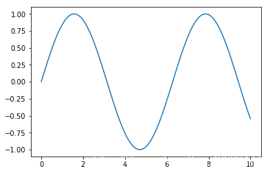
x = np.linspace(0,10,100)
x
array([ 0.        ,  0.1010101 ,  0.2020202 ,  0.3030303 ,  0.4040404 ,
        0.50505051,  0.60606061,  0.70707071,  0.80808081,  0.90909091,
        1.01010101,  1.11111111,  1.21212121,  1.31313131,  1.41414141,
        1.51515152,  1.61616162,  1.71717172,  1.81818182,  1.91919192,
        2.02020202,  2.12121212,  2.22222222,  2.32323232,  2.42424242,
        2.52525253,  2.62626263,  2.72727273,  2.82828283,  2.92929293,
        3.03030303,  3.13131313,  3.23232323,  3.33333333,  3.43434343,
        3.53535354,  3.63636364,  3.73737374,  3.83838384,  3.93939394,
        4.04040404,  4.14141414,  4.24242424,  4.34343434,  4.44444444,
        4.54545455,  4.64646465,  4.74747475,  4.84848485,  4.94949495,
        5.05050505,  5.15151515,  5.25252525,  5.35353535,  5.45454545,
        5.55555556,  5.65656566,  5.75757576,  5.85858586,  5.95959596,
        6.06060606,  6.16161616,  6.26262626,  6.36363636,  6.46464646,
        6.56565657,  6.66666667,  6.76767677,  6.86868687,  6.96969697,
        7.07070707,  7.17171717,  7.27272727,  7.37373737,  7.47474747,
        7.57575758,  7.67676768,  7.77777778,  7.87878788,  7.97979798,
        8.08080808,  8.18181818,  8.28282828,  8.38383838,  8.48484848,
        8.58585859,  8.68686869,  8.78787879,  8.88888889,  8.98989899,
        9.09090909,  9.19191919,  9.29292929,  9.39393939,  9.49494949,
        9.5959596 ,  9.6969697 ,  9.7979798 ,  9.8989899 , 10.        ])
y = np.sin(x)
y
array([ 0.        ,  0.10083842,  0.20064886,  0.2984138 ,  0.39313661,
        0.48385164,  0.56963411,  0.64960951,  0.72296256,  0.78894546,
        0.84688556,  0.8961922 ,  0.93636273,  0.96698762,  0.98775469,
        0.99845223,  0.99897117,  0.98930624,  0.96955595,  0.93992165,
        0.90070545,  0.85230712,  0.79522006,  0.73002623,  0.65739025,
        0.57805259,  0.49282204,  0.40256749,  0.30820902,  0.21070855,
        0.11106004,  0.01027934, -0.09060615, -0.19056796, -0.28858706,
       -0.38366419, -0.47483011, -0.56115544, -0.64176014, -0.7158225 ,
       -0.7825875 , -0.84137452, -0.89158426, -0.93270486, -0.96431712,
       -0.98609877, -0.99782778, -0.99938456, -0.99075324, -0.97202182,
       -0.94338126, -0.90512352, -0.85763861, -0.80141062, -0.73701276,
       -0.66510151, -0.58640998, -0.50174037, -0.41195583, -0.31797166,
       -0.22074597, -0.12126992, -0.0205576 ,  0.0803643 ,  0.18046693,
        0.27872982,  0.37415123,  0.46575841,  0.55261747,  0.63384295,
        0.7086068 ,  0.77614685,  0.83577457,  0.8868821 ,  0.92894843,
        0.96154471,  0.98433866,  0.99709789,  0.99969234,  0.99209556,
        0.97438499,  0.94674118,  0.90944594,  0.86287948,  0.8075165 ,
        0.74392141,  0.6727425 ,  0.59470541,  0.51060568,  0.42130064,
        0.32770071,  0.23076008,  0.13146699,  0.03083368, -0.07011396,
       -0.17034683, -0.26884313, -0.36459873, -0.45663749, -0.54402111])
plt.plot(x,y)
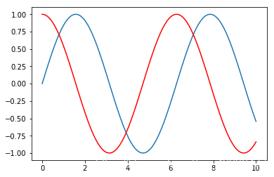
cosy = np.cos(x)
cosy.shape
(100,)
siny = y.copy()
plt.plot(x,siny)
plt.plot(x,cosy,color='red')
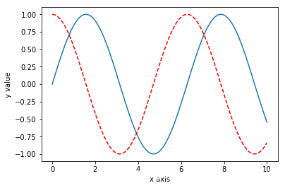
plt.plot(x,siny)
plt.plot(x,cosy,color='red',linestyle='--')
plt.xlim(-5,15)  #x轴的范围
plt.ylim(1,-1)  #y轴的范围

plt.plot(x,siny)
plt.plot(x,cosy,color='red',linestyle='--')
plt.axis([-1,11,-2,2])  #同时控制x,y轴的范围
在这里插入图片描述
plt.plot(x,siny)
plt.plot(x,cosy,color='red',linestyle='--')
plt.xlabel('x axis')
plt.ylabel('y value')
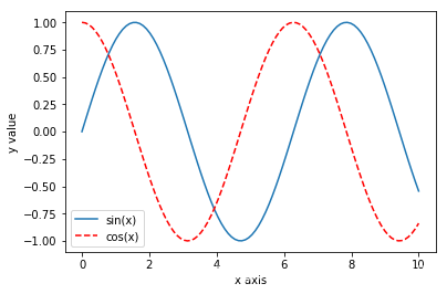
plt.plot(x,siny,label='sin(x)')
plt.plot(x,cosy,color='red',linestyle='--',label='cos(x)')
plt.xlabel('x axis')
plt.ylabel('y value')
plt.legend() #添加图示
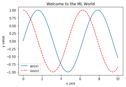
plt.plot(x,siny,label='sin(x)')
plt.plot(x,cosy,color='red',linestyle='--',label='cos(x)')
plt.xlabel('x axis')
plt.ylabel('y value')
plt.legend() #添加图示
plt.title("Welcome to the ML World") #添加标题
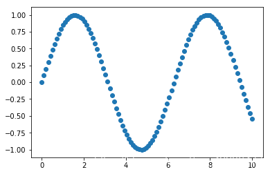
Scatter Plot
plt.scatter(x,siny)
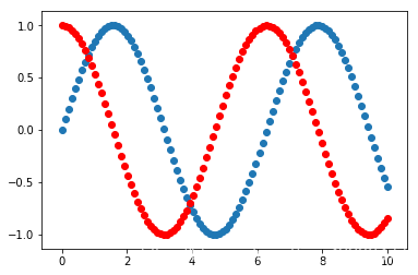
plt.scatter(x,siny)
plt.scatter(x,cosy,color='red')
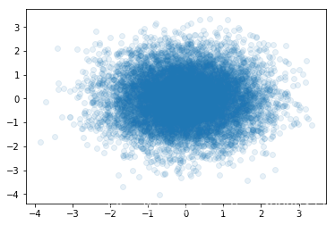
x = np.random.normal(0,1,10000) #服从均值为0,方差为1的正态分布
y = np.random.normal(0,1,10000)

plt.scatter(x,y,alpha=0.1)
读取数据和简单的数据探索
import numpy as np
import matplotlib as mpl
import matplotlib.pyplot as plt
from sklearn import datasets
iris = datasets.load_iris() #鸢尾花数据集
iris.keys()
dict_keys(['data', 'target', 'target_names', 'DESCR', 'feature_names', 'filename'])
print(iris.DESCR)
.. _iris_dataset:

Iris plants dataset
--------------------

**Data Set Characteristics:**

    :Number of Instances: 150 (50 in each of three classes)
    :Number of Attributes: 4 numeric, predictive attributes and the class
    :Attribute Information:
        - sepal length in cm
        - sepal width in cm
        - petal length in cm
        - petal width in cm
        - class:
                - Iris-Setosa
                - Iris-Versicolour
                - Iris-Virginica

    :Summary Statistics:

    ============== ==== ==== ======= ===== ====================
                    Min  Max   Mean    SD   Class Correlation
    ============== ==== ==== ======= ===== ====================
    sepal length:   4.3  7.9   5.84   0.83    0.7826
    sepal width:    2.0  4.4   3.05   0.43   -0.4194
    petal length:   1.0  6.9   3.76   1.76    0.9490  (high!)
    petal width:    0.1  2.5   1.20   0.76    0.9565  (high!)
    ============== ==== ==== ======= ===== ====================

    :Missing Attribute Values: None
    :Class Distribution: 33.3% for each of 3 classes.
    :Creator: R.A. Fisher
    :Donor: Michael Marshall (MARSHALL%[email protected])
    :Date: July, 1988

The famous Iris database, first used by Sir R.A. Fisher. The dataset is taken
from Fisher's paper. Note that it's the same as in R, but not as in the UCI
Machine Learning Repository, which has two wrong data points.

This is perhaps the best known database to be found in the
pattern recognition literature.  Fisher's paper is a classic in the field and
is referenced frequently to this day.  (See Duda & Hart, for example.)  The
data set contains 3 classes of 50 instances each, where each class refers to a
type of iris plant.  One class is linearly separable from the other 2; the
latter are NOT linearly separable from each other.

.. topic:: References

   - Fisher, R.A. "The use of multiple measurements in taxonomic problems"
     Annual Eugenics, 7, Part II, 179-188 (1936); also in "Contributions to
     Mathematical Statistics" (John Wiley, NY, 1950).
   - Duda, R.O., & Hart, P.E. (1973) Pattern Classification and Scene Analysis.
     (Q327.D83) John Wiley & Sons.  ISBN 0-471-22361-1.  See page 218.
   - Dasarathy, B.V. (1980) "Nosing Around the Neighborhood: A New System
     Structure and Classification Rule for Recognition in Partially Exposed
     Environments".  IEEE Transactions on Pattern Analysis and Machine
     Intelligence, Vol. PAMI-2, No. 1, 67-71.
   - Gates, G.W. (1972) "The Reduced Nearest Neighbor Rule".  IEEE Transactions
     on Information Theory, May 1972, 431-433.
   - See also: 1988 MLC Proceedings, 54-64.  Cheeseman et al"s AUTOCLASS II
     conceptual clustering system finds 3 classes in the data.
   - Many, many more ...
iris.data
array([[5.1, 3.5, 1.4, 0.2],
       [4.9, 3. , 1.4, 0.2],
       [4.7, 3.2, 1.3, 0.2],
       [4.6, 3.1, 1.5, 0.2],
       [5. , 3.6, 1.4, 0.2],
       [5.4, 3.9, 1.7, 0.4],
       [4.6, 3.4, 1.4, 0.3],
       [5. , 3.4, 1.5, 0.2],
       [4.4, 2.9, 1.4, 0.2],
       [4.9, 3.1, 1.5, 0.1],
       [5.4, 3.7, 1.5, 0.2],
       [4.8, 3.4, 1.6, 0.2],
       [4.8, 3. , 1.4, 0.1],
       [4.3, 3. , 1.1, 0.1],
       [5.8, 4. , 1.2, 0.2],
       [5.7, 4.4, 1.5, 0.4],
       [5.4, 3.9, 1.3, 0.4],
       [5.1, 3.5, 1.4, 0.3],
       [5.7, 3.8, 1.7, 0.3],
       [5.1, 3.8, 1.5, 0.3],
       [5.4, 3.4, 1.7, 0.2],
       [5.1, 3.7, 1.5, 0.4],
       [4.6, 3.6, 1. , 0.2],
       [5.1, 3.3, 1.7, 0.5],
       [4.8, 3.4, 1.9, 0.2],
       [5. , 3. , 1.6, 0.2],
       [5. , 3.4, 1.6, 0.4],
       [5.2, 3.5, 1.5, 0.2],
       [5.2, 3.4, 1.4, 0.2],
       [4.7, 3.2, 1.6, 0.2],
       [4.8, 3.1, 1.6, 0.2],
       [5.4, 3.4, 1.5, 0.4],
       [5.2, 4.1, 1.5, 0.1],
       [5.5, 4.2, 1.4, 0.2],
       [4.9, 3.1, 1.5, 0.2],
       [5. , 3.2, 1.2, 0.2],
       [5.5, 3.5, 1.3, 0.2],
       [4.9, 3.6, 1.4, 0.1],
       [4.4, 3. , 1.3, 0.2],
       [5.1, 3.4, 1.5, 0.2],
       [5. , 3.5, 1.3, 0.3],
       [4.5, 2.3, 1.3, 0.3],
       [4.4, 3.2, 1.3, 0.2],
       [5. , 3.5, 1.6, 0.6],
       [5.1, 3.8, 1.9, 0.4],
       [4.8, 3. , 1.4, 0.3],
       [5.1, 3.8, 1.6, 0.2],
       [4.6, 3.2, 1.4, 0.2],
       [5.3, 3.7, 1.5, 0.2],
       [5. , 3.3, 1.4, 0.2],
       [7. , 3.2, 4.7, 1.4],
       [6.4, 3.2, 4.5, 1.5],
       [6.9, 3.1, 4.9, 1.5],
       [5.5, 2.3, 4. , 1.3],
       [6.5, 2.8, 4.6, 1.5],
       [5.7, 2.8, 4.5, 1.3],
       [6.3, 3.3, 4.7, 1.6],
       [4.9, 2.4, 3.3, 1. ],
       [6.6, 2.9, 4.6, 1.3],
       [5.2, 2.7, 3.9, 1.4],
       [5. , 2. , 3.5, 1. ],
       [5.9, 3. , 4.2, 1.5],
       [6. , 2.2, 4. , 1. ],
       [6.1, 2.9, 4.7, 1.4],
       [5.6, 2.9, 3.6, 1.3],
       [6.7, 3.1, 4.4, 1.4],
       [5.6, 3. , 4.5, 1.5],
       [5.8, 2.7, 4.1, 1. ],
       [6.2, 2.2, 4.5, 1.5],
       [5.6, 2.5, 3.9, 1.1],
       [5.9, 3.2, 4.8, 1.8],
       [6.1, 2.8, 4. , 1.3],
       [6.3, 2.5, 4.9, 1.5],
       [6.1, 2.8, 4.7, 1.2],
       [6.4, 2.9, 4.3, 1.3],
       [6.6, 3. , 4.4, 1.4],
       [6.8, 2.8, 4.8, 1.4],
       [6.7, 3. , 5. , 1.7],
       [6. , 2.9, 4.5, 1.5],
       [5.7, 2.6, 3.5, 1. ],
       [5.5, 2.4, 3.8, 1.1],
       [5.5, 2.4, 3.7, 1. ],
       [5.8, 2.7, 3.9, 1.2],
       [6. , 2.7, 5.1, 1.6],
       [5.4, 3. , 4.5, 1.5],
       [6. , 3.4, 4.5, 1.6],
       [6.7, 3.1, 4.7, 1.5],
       [6.3, 2.3, 4.4, 1.3],
       [5.6, 3. , 4.1, 1.3],
       [5.5, 2.5, 4. , 1.3],
       [5.5, 2.6, 4.4, 1.2],
       [6.1, 3. , 4.6, 1.4],
       [5.8, 2.6, 4. , 1.2],
       [5. , 2.3, 3.3, 1. ],
       [5.6, 2.7, 4.2, 1.3],
       [5.7, 3. , 4.2, 1.2],
       [5.7, 2.9, 4.2, 1.3],
       [6.2, 2.9, 4.3, 1.3],
       [5.1, 2.5, 3. , 1.1],
       [5.7, 2.8, 4.1, 1.3],
       [6.3, 3.3, 6. , 2.5],
       [5.8, 2.7, 5.1, 1.9],
       [7.1, 3. , 5.9, 2.1],
       [6.3, 2.9, 5.6, 1.8],
       [6.5, 3. , 5.8, 2.2],
       [7.6, 3. , 6.6, 2.1],
       [4.9, 2.5, 4.5, 1.7],
       [7.3, 2.9, 6.3, 1.8],
       [6.7, 2.5, 5.8, 1.8],
       [7.2, 3.6, 6.1, 2.5],
       [6.5, 3.2, 5.1, 2. ],
       [6.4, 2.7, 5.3, 1.9],
       [6.8, 3. , 5.5, 2.1],
       [5.7, 2.5, 5. , 2. ],
       [5.8, 2.8, 5.1, 2.4],
       [6.4, 3.2, 5.3, 2.3],
       [6.5, 3. , 5.5, 1.8],
       [7.7, 3.8, 6.7, 2.2],
       [7.7, 2.6, 6.9, 2.3],
       [6. , 2.2, 5. , 1.5],
       [6.9, 3.2, 5.7, 2.3],
       [5.6, 2.8, 4.9, 2. ],
       [7.7, 2.8, 6.7, 2. ],
       [6.3, 2.7, 4.9, 1.8],
       [6.7, 3.3, 5.7, 2.1],
       [7.2, 3.2, 6. , 1.8],
       [6.2, 2.8, 4.8, 1.8],
       [6.1, 3. , 4.9, 1.8],
       [6.4, 2.8, 5.6, 2.1],
       [7.2, 3. , 5.8, 1.6],
       [7.4, 2.8, 6.1, 1.9],
       [7.9, 3.8, 6.4, 2. ],
       [6.4, 2.8, 5.6, 2.2],
       [6.3, 2.8, 5.1, 1.5],
       [6.1, 2.6, 5.6, 1.4],
       [7.7, 3. , 6.1, 2.3],
       [6.3, 3.4, 5.6, 2.4],
       [6.4, 3.1, 5.5, 1.8],
       [6. , 3. , 4.8, 1.8],
       [6.9, 3.1, 5.4, 2.1],
       [6.7, 3.1, 5.6, 2.4],
       [6.9, 3.1, 5.1, 2.3],
       [5.8, 2.7, 5.1, 1.9],
       [6.8, 3.2, 5.9, 2.3],
       [6.7, 3.3, 5.7, 2.5],
       [6.7, 3. , 5.2, 2.3],
       [6.3, 2.5, 5. , 1.9],
       [6.5, 3. , 5.2, 2. ],
       [6.2, 3.4, 5.4, 2.3],
       [5.9, 3. , 5.1, 1.8]])
iris.data.shape
(150, 4)
iris.feature_names
['sepal length (cm)',
 'sepal width (cm)',
 'petal length (cm)',
 'petal width (cm)']
iris.target
array([0, 0, 0, 0, 0, 0, 0, 0, 0, 0, 0, 0, 0, 0, 0, 0, 0, 0, 0, 0, 0, 0,
       0, 0, 0, 0, 0, 0, 0, 0, 0, 0, 0, 0, 0, 0, 0, 0, 0, 0, 0, 0, 0, 0,
       0, 0, 0, 0, 0, 0, 1, 1, 1, 1, 1, 1, 1, 1, 1, 1, 1, 1, 1, 1, 1, 1,
       1, 1, 1, 1, 1, 1, 1, 1, 1, 1, 1, 1, 1, 1, 1, 1, 1, 1, 1, 1, 1, 1,
       1, 1, 1, 1, 1, 1, 1, 1, 1, 1, 1, 1, 2, 2, 2, 2, 2, 2, 2, 2, 2, 2,
       2, 2, 2, 2, 2, 2, 2, 2, 2, 2, 2, 2, 2, 2, 2, 2, 2, 2, 2, 2, 2, 2,
       2, 2, 2, 2, 2, 2, 2, 2, 2, 2, 2, 2, 2, 2, 2, 2, 2, 2])
iris.target.shape
(150,)
iris.target_names
array(['setosa', 'versicolor', 'virginica'], dtype='<U10')
X = iris.data[:,:2] #取前两列
X
array([[5.1, 3.5],
       [4.9, 3. ],
       [4.7, 3.2],
       [4.6, 3.1],
       [5. , 3.6],
       [5.4, 3.9],
       [4.6, 3.4],
       [5. , 3.4],
       [4.4, 2.9],
       [4.9, 3.1],
       [5.4, 3.7],
       [4.8, 3.4],
       [4.8, 3. ],
       [4.3, 3. ],
       [5.8, 4. ],
       [5.7, 4.4],
       [5.4, 3.9],
       [5.1, 3.5],
       [5.7, 3.8],
       [5.1, 3.8],
       [5.4, 3.4],
       [5.1, 3.7],
       [4.6, 3.6],
       [5.1, 3.3],
       [4.8, 3.4],
       [5. , 3. ],
       [5. , 3.4],
       [5.2, 3.5],
       [5.2, 3.4],
       [4.7, 3.2],
       [4.8, 3.1],
       [5.4, 3.4],
       [5.2, 4.1],
       [5.5, 4.2],
       [4.9, 3.1],
       [5. , 3.2],
       [5.5, 3.5],
       [4.9, 3.6],
       [4.4, 3. ],
       [5.1, 3.4],
       [5. , 3.5],
       [4.5, 2.3],
       [4.4, 3.2],
       [5. , 3.5],
       [5.1, 3.8],
       [4.8, 3. ],
       [5.1, 3.8],
       [4.6, 3.2],
       [5.3, 3.7],
       [5. , 3.3],
       [7. , 3.2],
       [6.4, 3.2],
       [6.9, 3.1],
       [5.5, 2.3],
       [6.5, 2.8],
       [5.7, 2.8],
       [6.3, 3.3],
       [4.9, 2.4],
       [6.6, 2.9],
       [5.2, 2.7],
       [5. , 2. ],
       [5.9, 3. ],
       [6. , 2.2],
       [6.1, 2.9],
       [5.6, 2.9],
       [6.7, 3.1],
       [5.6, 3. ],
       [5.8, 2.7],
       [6.2, 2.2],
       [5.6, 2.5],
       [5.9, 3.2],
       [6.1, 2.8],
       [6.3, 2.5],
       [6.1, 2.8],
       [6.4, 2.9],
       [6.6, 3. ],
       [6.8, 2.8],
       [6.7, 3. ],
       [6. , 2.9],
       [5.7, 2.6],
       [5.5, 2.4],
       [5.5, 2.4],
       [5.8, 2.7],
       [6. , 2.7],
       [5.4, 3. ],
       [6. , 3.4],
       [6.7, 3.1],
       [6.3, 2.3],
       [5.6, 3. ],
       [5.5, 2.5],
       [5.5, 2.6],
       [6.1, 3. ],
       [5.8, 2.6],
       [5. , 2.3],
       [5.6, 2.7],
       [5.7, 3. ],
       [5.7, 2.9],
       [6.2, 2.9],
       [5.1, 2.5],
       [5.7, 2.8],
       [6.3, 3.3],
       [5.8, 2.7],
       [7.1, 3. ],
       [6.3, 2.9],
       [6.5, 3. ],
       [7.6, 3. ],
       [4.9, 2.5],
       [7.3, 2.9],
       [6.7, 2.5],
       [7.2, 3.6],
       [6.5, 3.2],
       [6.4, 2.7],
       [6.8, 3. ],
       [5.7, 2.5],
       [5.8, 2.8],
       [6.4, 3.2],
       [6.5, 3. ],
       [7.7, 3.8],
       [7.7, 2.6],
       [6. , 2.2],
       [6.9, 3.2],
       [5.6, 2.8],
       [7.7, 2.8],
       [6.3, 2.7],
       [6.7, 3.3],
       [7.2, 3.2],
       [6.2, 2.8],
       [6.1, 3. ],
       [6.4, 2.8],
       [7.2, 3. ],
       [7.4, 2.8],
       [7.9, 3.8],
       [6.4, 2.8],
       [6.3, 2.8],
       [6.1, 2.6],
       [7.7, 3. ],
       [6.3, 3.4],
       [6.4, 3.1],
       [6. , 3. ],
       [6.9, 3.1],
       [6.7, 3.1],
       [6.9, 3.1],
       [5.8, 2.7],
       [6.8, 3.2],
       [6.7, 3.3],
       [6.7, 3. ],
       [6.3, 2.5],
       [6.5, 3. ],
       [6.2, 3.4],
       [5.9, 3. ]])
X.shape
(150, 2)
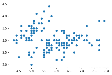
plt.scatter(X[:,0],X[:,1]) #分别取矩阵中的第0列、第1列作为x轴、y轴
plt.show()
y = iris.target
array([0, 0, 0, 0, 0, 0, 0, 0, 0, 0, 0, 0, 0, 0, 0, 0, 0, 0, 0, 0, 0, 0,
       0, 0, 0, 0, 0, 0, 0, 0, 0, 0, 0, 0, 0, 0, 0, 0, 0, 0, 0, 0, 0, 0,
       0, 0, 0, 0, 0, 0, 1, 1, 1, 1, 1, 1, 1, 1, 1, 1, 1, 1, 1, 1, 1, 1,
       1, 1, 1, 1, 1, 1, 1, 1, 1, 1, 1, 1, 1, 1, 1, 1, 1, 1, 1, 1, 1, 1,
       1, 1, 1, 1, 1, 1, 1, 1, 1, 1, 1, 1, 2, 2, 2, 2, 2, 2, 2, 2, 2, 2,
       2, 2, 2, 2, 2, 2, 2, 2, 2, 2, 2, 2, 2, 2, 2, 2, 2, 2, 2, 2, 2, 2,
       2, 2, 2, 2, 2, 2, 2, 2, 2, 2, 2, 2, 2, 2, 2, 2, 2, 2])
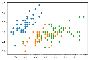
plt.scatter(X[y==0,0],X[y==0,1])
plt.scatter(X[y==1,0],X[y==1,1])
plt.scatter(X[y==2,0],X[y==2,1])
plt.show()
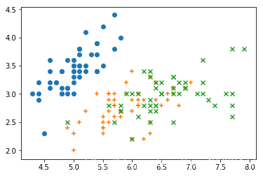
plt.scatter(X[y==0,0],X[y==0,1],marker='o')
plt.scatter(X[y==1,0],X[y==1,1],marker='+')
plt.scatter(X[y==2,0],X[y==2,1],marker='x')#添加散点样式
plt.show()
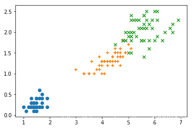
X = iris.data[:,2:] #取后两列
plt.scatter(X[y==0,0],X[y==0,1],marker='o')
plt.scatter(X[y==1,0],X[y==1,1],marker='+')
plt.scatter(X[y==2,0],X[y==2,1],marker='x')#添加散点样式
plt.show()