版权声明:可以随意转载→_→ https://blog.csdn.net/ds19991999/article/details/81294905
Matplotlib 基础
Matplotlib是一个类似Matlab的工具包,主要用来画图,主页地址为:Matplotlib
# 导入 matplotlib 和 numpy:
%pylab
Using matplotlib backend: TkAgg
Populating the interactive namespace from numpy and matplotlib
plot 二维图
plot(y)
plot(x, y)
plot(x, y, format_string)
只给定 y 值,默认以下标为 x 轴:
%matplotlib inline
x = linspace(0,2*pi,50)
plot(sin(x)) # 没有给定x,则范围为0-50
[<matplotlib.lines.Line2D at 0x9d69b50>]

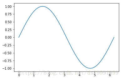
# 给定x和y值
plot(x, sin(x)) # 给定x,则范围为0-2pi
[<matplotlib.lines.Line2D at 0x9f4c050>]
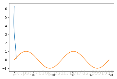
# 多条数据线
plot(sin(x)/x,
     x,sin(2*x))
d:\python\lib\site-packages\ipykernel_launcher.py:2: RuntimeWarning: invalid value encountered in divide
[<matplotlib.lines.Line2D at 0xa186ed0>,
<matplotlib.lines.Line2D at 0xa186fb0>]
# 使用字符串,给定线条参数:
plot(x, sin(x), 'r-^')
[<matplotlib.lines.Line2D at 0xb158070>]

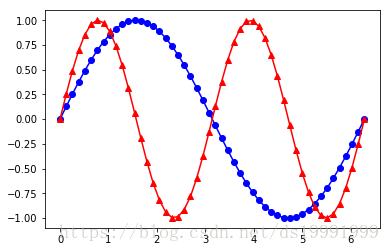
# 多线条:
plot(x,sin(x),'b-o',
    x,sin(2*x),'r-^')
[<matplotlib.lines.Line2D at 0xb255530>,
<matplotlib.lines.Line2D at 0xb255650>]
scatter散点图
scatter(x, y)
scatter(x, y, size)
scatter(x, y, size, color)
假设我们想画二维散点图:
plot(x, sin(x), 'bo')[<matplotlib.lines.Line2D at 0xb392b10>]
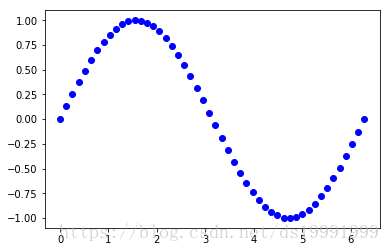
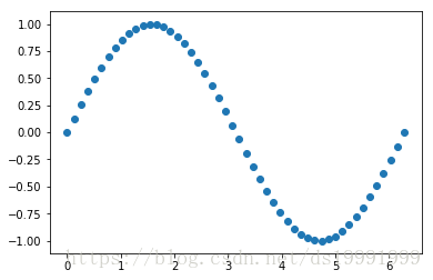
# 使用 scatter 达到同样的效果
scatter(x, sin(x))
<matplotlib.collections.PathCollection at 0xb392bd0>
# scatter函数与Matlab的用法相同,还可以指定它的大小,颜色等参数
x = rand(200)
y = rand(200)
size = rand(200) * 30
color = rand(200)
scatter(x, y, size, color)
# 显示颜色条
colorbar()
<matplotlib.colorbar.Colorbar at 0xb6fea90>

多图
# 使用figure()命令产生新的图像:
t = linspace(0, 2*pi, 50)
x = sin(t)
y = cos(t)
figure()
plot(x)
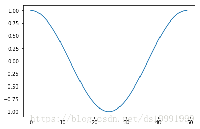
figure()
plot(y)[<matplotlib.lines.Line2D at 0xb530590>]

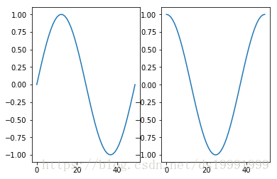
# 或者使用 subplot 在一幅图中画多幅子图:
# subplot(row, column, index)
subplot(1, 2, 1)
plot(x)
subplot(1, 2, 2)
plot(y)
[<matplotlib.lines.Line2D at 0xb5c7410>]
向图中添加数据
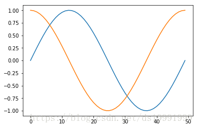
# 默认多次 plot 会叠加:
plot(x)
plot(y)
[<matplotlib.lines.Line2D at 0xe7b9a90>]
# 跟Matlab类似用 hold(False)关掉,这样新图会将原图覆盖:
plot(x)
hold(False)
plot(y)
# 恢复原来设定
hold(True)
d:\python\lib\site-packages\ipykernel_launcher.py:3: MatplotlibDeprecationWarning: pyplot.hold is deprecated.
Future behavior will be consistent with the long-time default:
plot commands add elements without first clearing the
Axes and/or Figure.
This is separate from the ipykernel package so we can avoid doing imports until
d:\python\lib\site-packages\matplotlib\__init__.py:911: MatplotlibDeprecationWarning: axes.hold is deprecated. Please remove it from your matplotlibrc and/or style files.
mplDeprecation)
d:\python\lib\site-packages\matplotlib\rcsetup.py:156: MatplotlibDeprecationWarning: axes.hold is deprecated, will be removed in 3.0
mplDeprecation)
d:\python\lib\site-packages\ipykernel_launcher.py:6: MatplotlibDeprecationWarning: pyplot.hold is deprecated.
Future behavior will be consistent with the long-time default:
plot commands add elements without first clearing the
Axes and/or Figure.

标签
# 可以在 plot 中加入 label ,使用 legend 加上图例:
plot(x, label='sin')
plot(y, label='cos')
legend()
<matplotlib.legend.Legend at 0xeb1b7f0>
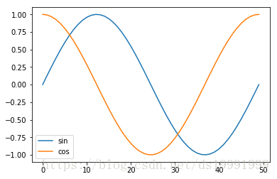
# 或者直接在 legend中加入:
plot(x)
plot(y)
legend(['sin', 'cos'])
<matplotlib.legend.Legend at 0xebc21b0>

坐标轴,标题,网格
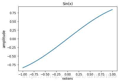
# 可以设置坐标轴的标签和标题:
plot(x, sin(x))
xlabel('radians')
# 可以设置字体大小
ylabel('amplitude', fontsize='large')
title('Sin(x)')
Text(0.5,1,'Sin(x)')
# 用 'grid()' 来显示网格:
plot(x, sin(x))
xlabel('radians')
ylabel('amplitude', fontsize='large')
title('Sin(x)')
grid()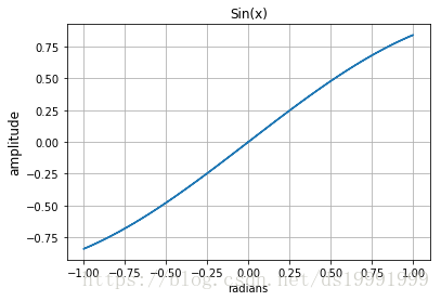
清除、关闭图像
清除已有的图像使用:clf()
关闭当前图像:close()
关闭所有图像:close('all')
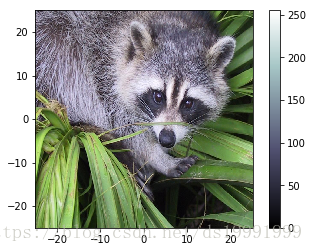
imshow 显示图片
这里需要注意,之前misc中的示例图片被删除了,查看帮助文档,发现换成了另一个名称

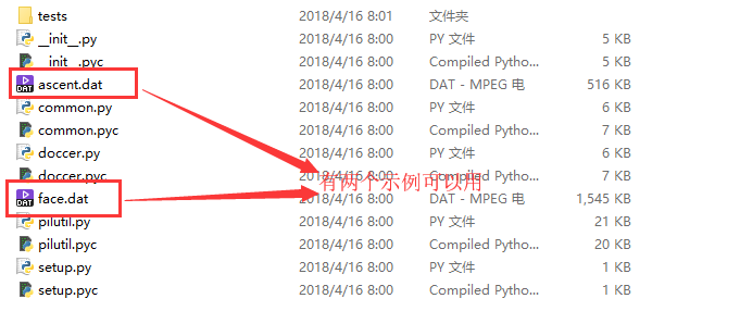
# 导入lena图片
from scipy.misc import face,ascent
img1 = face()
img2 = ascent()
imshow(img1,
# 设置坐标范围
extent = [-25, 25, -25, 25],
# 设置colormap
cmap = cm.bone)
colorbar()<matplotlib.colorbar.Colorbar at 0x10639950>
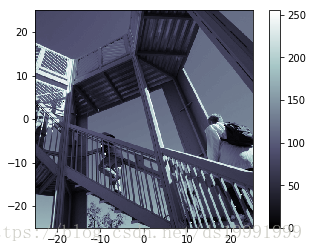
imshow(img2,
# 设置坐标范围
extent = [-25, 25, -25, 25],
# 设置colormap
cmap = cm.bone)
colorbar()<matplotlib.colorbar.Colorbar at 0x1092a030>
# 看一下img的数据
print 'face:\n',img1
print 'ascent:\n',img2face:
[[[121 112 131]
[138 129 148]
[153 144 165]
...
[119 126 74]
[131 136 82]
[139 144 90]]
[[ 89 82 100]
[110 103 121]
[130 122 143]
...
[118 125 71]
[134 141 87]
[146 153 99]]
[[ 73 66 84]
[ 94 87 105]
[115 108 126]
...
[117 126 71]
[133 142 87]
[144 153 98]]
...
[[ 87 106 76]
[ 94 110 81]
[107 124 92]
...
[120 158 97]
[119 157 96]
[119 158 95]]
[[ 85 101 72]
[ 95 111 82]
[112 127 96]
...
[121 157 96]
[120 156 94]
[120 156 94]]
[[ 85 101 74]
[ 97 113 84]
[111 126 97]
...
[120 156 95]
[119 155 93]
[118 154 92]]]
ascent:
[[ 83 83 83 ... 117 117 117]
[ 82 82 83 ... 117 117 117]
[ 80 81 83 ... 117 117 117]
...
[178 178 178 ... 57 59 57]
[178 178 178 ... 56 57 57]
[178 178 178 ... 57 57 58]]
imshow??# 这里 cm 表示 colormap,可以看它的种类:
dir(cm)[u'Accent',
u'Accent_r',
u'Blues',
u'Blues_r',
u'BrBG',
u'BrBG_r',
u'BuGn',
u'BuGn_r',
u'BuPu',
u'BuPu_r',
u'CMRmap',
u'CMRmap_r',
u'Dark2',
u'Dark2_r',
u'GnBu',
u'GnBu_r',
u'Greens',
u'Greens_r',
u'Greys',
u'Greys_r',
'LUTSIZE',
u'OrRd',
u'OrRd_r',
u'Oranges',
u'Oranges_r',
u'PRGn',
u'PRGn_r',
u'Paired',
u'Paired_r',
u'Pastel1',
u'Pastel1_r',
u'Pastel2',
u'Pastel2_r',
u'PiYG',
u'PiYG_r',
u'PuBu',
u'PuBuGn',
u'PuBuGn_r',
u'PuBu_r',
u'PuOr',
u'PuOr_r',
u'PuRd',
u'PuRd_r',
u'Purples',
u'Purples_r',
u'RdBu',
u'RdBu_r',
u'RdGy',
u'RdGy_r',
u'RdPu',
u'RdPu_r',
u'RdYlBu',
u'RdYlBu_r',
u'RdYlGn',
u'RdYlGn_r',
u'Reds',
u'Reds_r',
'ScalarMappable',
u'Set1',
u'Set1_r',
u'Set2',
u'Set2_r',
u'Set3',
u'Set3_r',
u'Spectral',
u'Spectral_r',
u'Wistia',
u'Wistia_r',
u'YlGn',
u'YlGnBu',
u'YlGnBu_r',
u'YlGn_r',
u'YlOrBr',
u'YlOrBr_r',
u'YlOrRd',
u'YlOrRd_r',
'__builtins__',
'__doc__',
'__file__',
'__name__',
'__package__',
'_generate_cmap',
'_reverse_cmap_spec',
'_reverser',
'absolute_import',
u'afmhot',
u'afmhot_r',
u'autumn',
u'autumn_r',
u'binary',
u'binary_r',
u'bone',
u'bone_r',
u'brg',
u'brg_r',
u'bwr',
u'bwr_r',
'cbook',
'cividis',
'cividis_r',
'cmap_d',
'cmapname',
'cmaps_listed',
'colors',
u'cool',
u'cool_r',
u'coolwarm',
u'coolwarm_r',
u'copper',
u'copper_r',
u'cubehelix',
u'cubehelix_r',
'datad',
'division',
u'flag',
u'flag_r',
'get_cmap',
u'gist_earth',
u'gist_earth_r',
u'gist_gray',
u'gist_gray_r',
u'gist_heat',
u'gist_heat_r',
u'gist_ncar',
u'gist_ncar_r',
u'gist_rainbow',
u'gist_rainbow_r',
u'gist_stern',
u'gist_stern_r',
u'gist_yarg',
u'gist_yarg_r',
u'gnuplot',
u'gnuplot2',
u'gnuplot2_r',
u'gnuplot_r',
u'gray',
u'gray_r',
u'hot',
u'hot_r',
u'hsv',
u'hsv_r',
'inferno',
'inferno_r',
u'jet',
u'jet_r',
'ma',
'magma',
'magma_r',
'mpl',
u'nipy_spectral',
u'nipy_spectral_r',
'np',
u'ocean',
u'ocean_r',
u'pink',
u'pink_r',
'plasma',
'plasma_r',
'print_function',
u'prism',
u'prism_r',
u'rainbow',
u'rainbow_r',
'register_cmap',
'revcmap',
u'seismic',
u'seismic_r',
'six',
u'spring',
u'spring_r',
u'summer',
u'summer_r',
u'tab10',
u'tab10_r',
u'tab20',
u'tab20_r',
u'tab20b',
u'tab20b_r',
u'tab20c',
u'tab20c_r',
u'terrain',
u'terrain_r',
'unicode_literals',
'viridis',
'viridis_r',
u'winter',
u'winter_r']
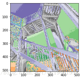
imshow(img2, cmap=cm.tab20c_r)<matplotlib.image.AxesImage at 0x10bdd9b0>
从脚本中运行
在脚本中使用 plot 时,通常图像是不会直接显示的,需要增加 show() 选项,只有在遇到 show() 命令之后,图像才会显示。
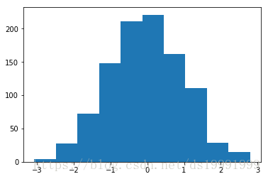
直方图
# 从高斯分布随机生成1000个点得到的直方图:
hist(randn(1000))(array([ 4., 27., 72., 148., 211., 221., 162., 111., 29., 15.]),
array([-3.06945987, -2.48284754, -1.89623522, -1.3096229 , -0.72301058,
-0.13639825, 0.45021407, 1.03682639, 1.62343871, 2.21005103,
2.79666336]),
<a list of 10 Patch objects>)
"""
==================
A simple Fill plot
==================
This example showcases the most basic fill plot a user can do with matplotlib.
"""
import numpy as np
import matplotlib.pyplot as plt
x = np.linspace(0, 1, 500)
y = np.sin(4 * np.pi * x) * np.exp(-5 * x)
fig, ax = plt.subplots()
ax.fill(x, y, zorder=10)
ax.grid(True, zorder=5)
plt.show()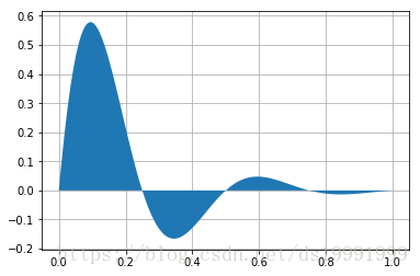
"""
========================
A more complex fill demo
========================
In addition to the basic fill plot, this demo shows a few optional features:
* Multiple curves with a single command.
* Setting the fill color.
* Setting the opacity (alpha value).
"""
import numpy as np
import matplotlib.pyplot as plt
x = np.linspace(0, 2 * np.pi, 500)
y1 = np.sin(x)
y2 = np.sin(3 * x)
fig, ax = plt.subplots()
ax.fill(x, y1, 'b', x, y2, 'r', alpha=0.3)
plt.show()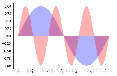
总结
# 导入 matplotlib 和 numpy:
%pylab
%matplotlib inline
x = linspace(0,2*pi,50)
plot(sin(x)) # 没有给定x,则范围为0-50
# 给定x和y值
plot(x, sin(x)) # 给定x,则范围为0-2pi
# 多条数据线
plot(x,sin(x),
x,sin(2*x))
# 使用字符串,给定线条参数:
plot(x, sin(x), 'r-^')
# 多线条:
plot(x,sin(x),'b-o',
x,sin(2*x),'r-^')
# 假设我们想画二维散点图:
plot(x, sin(x), 'bo')
# 使用 scatter 达到同样的效果
scatter(x, sin(x))
# scatter函数与Matlab的用法相同,还可以指定它的大小,颜色等参数
x = rand(200)
y = rand(200)
size = rand(200) * 30
color = rand(200)
scatter(x, y, size, color)
# 显示颜色条
colorbar()
# 使用figure()命令产生新的图像:
t = linspace(0, 2*pi, 50)
x = sin(t)
y = cos(t)
figure()
plot(x)
figure()
plot(y)
# 或者使用 subplot 在一幅图中画多幅子图:
# subplot(row, column, index)
subplot(1, 2, 1)
plot(x)
subplot(1, 2, 2)
plot(y)
# 默认多次 plot 会叠加:
plot(x)
plot(y)
# 跟Matlab类似用 hold(False)关掉,这样新图会将原图覆盖:
plot(x)
hold(False)
plot(y)
# 恢复原来设定
hold(True)
# 可以在 plot 中加入 label ,使用 legend 加上图例:
plot(x, label='sin')
plot(y, label='cos')
legend()
# 或者直接在 legend中加入:
plot(x)
plot(y)
legend(['sin', 'cos'])
# 可以设置坐标轴的标签和标题:
plot(x, sin(x))
xlabel('radians')
# 可以设置字体大小
ylabel('amplitude', fontsize='large')
title('Sin(x)')
# 用 'grid()' 来显示网格:
grid()
# 导入lena图片
from scipy.misc import face,ascent
img1 = face()
img2 = ascent()
# 显示图片
imshow(img1,
       # 设置坐标范围
      extent = [-25, 25, -25, 25],
       # 设置colormap
      cmap = cm.bone)
colorbar()
# 在脚本中使用 plot 时,通常图像是不会直接显示的,需要增加 show() 选项,只有在遇到 show() 命令之后,图像才会显示。
# 从高斯分布随机生成1000个点得到的直方图:
hist(randn(1000))
# 查阅帮助 <模块或者函数名>??