一、数据可视化的概念
数据可视化是指将大型数据集中的数据以图形图像形式表示,并利用数据分析和开发工具发现其中未知信息的处理过程。数据可视化技术的基本思想是将数据库中每一个数据项作为单个图元素表示,大量的数据集构成数据图像,同时将数据的各个属性值以多维数据的形式表示,可以从不同的维度观察数据,从而对数据进行更深入的观察和分析。
二、数据可视化的重要作用
①观测、跟踪数据。利用变化的数据生成实时变化的可视化图表,可以让人们一眼看出各种参数的动态变化过程,有效跟踪各种参数值。 ②分析数据。利用可视化技术,实时呈现当前分析结果,引导用户参与分析过程,根据用户反馈信息执行后续分析操作,完成用户与分析算法的全程交互,实现数据分析算法与用户领域知识的完美结合。 ③辅助理解数据。帮助普通用户更快、更准确地理解数据背后的定义。 ④增强数据吸引力。枯燥的数据被制成具有强大视觉冲击力和说服力的图像,可以大大增强读者的阅读兴趣。
三、Iris数据集的 Fisher线性分类
sklearn的datasets(鸢尾花数据集),此数据集包含四列,分别是鸢尾花的四个特征:
sepal length (cm)——花萼长度
sepal width (cm)——花萼宽度
petal length (cm)——花瓣长度
petal width (cm)——花瓣宽度
- 导入数据,此数据集在sklearn库中存在
from sklearn import datasets
import pandas as pd
import matplotlib.pyplot as plt
import numpy as np
import seaborn as sns
from mpl_toolkits.mplot3d import Axes3D
iris = datasets.load_iris()
- 导入的iris数据集
data1=pd.DataFrame(np.concatenate((iris.data,iris.target.reshape(150,1)),axis=1),
                           columns=np.append(iris.feature_names,'target'))
data1
运行结果
| sepal length (cm) | sepal width (cm) | petal length (cm) | petal width (cm) | target | |
|---|---|---|---|---|---|
| 0 | 5.1 | 3.5 | 1.4 | 0.2 | 0.0 |
| 1 | 4.9 | 3.0 | 1.4 | 0.2 | 0.0 |
| 2 | 4.7 | 3.2 | 1.3 | 0.2 | 0.0 |
| 3 | 4.6 | 3.1 | 1.5 | 0.2 | 0.0 |
| 4 | 5.0 | 3.6 | 1.4 | 0.2 | 0.0 |
| 5 | 5.4 | 3.9 | 1.7 | 0.4 | 0.0 |
| 6 | 4.6 | 3.4 | 1.4 | 0.3 | 0.0 |
| 7 | 5.0 | 3.4 | 1.5 | 0.2 | 0.0 |
| 8 | 4.4 | 2.9 | 1.4 | 0.2 | 0.0 |
| 9 | 4.9 | 3.1 | 1.5 | 0.1 | 0.0 |
| 10 | 5.4 | 3.7 | 1.5 | 0.2 | 0.0 |
| 11 | 4.8 | 3.4 | 1.6 | 0.2 | 0.0 |
| 12 | 4.8 | 3.0 | 1.4 | 0.1 | 0.0 |
| 13 | 4.3 | 3.0 | 1.1 | 0.1 | 0.0 |
| 14 | 5.8 | 4.0 | 1.2 | 0.2 | 0.0 |
| 15 | 5.7 | 4.4 | 1.5 | 0.4 | 0.0 |
| 16 | 5.4 | 3.9 | 1.3 | 0.4 | 0.0 |
| 17 | 5.1 | 3.5 | 1.4 | 0.3 | 0.0 |
| 18 | 5.7 | 3.8 | 1.7 | 0.3 | 0.0 |
| 19 | 5.1 | 3.8 | 1.5 | 0.3 | 0.0 |
| 20 | 5.4 | 3.4 | 1.7 | 0.2 | 0.0 |
| 21 | 5.1 | 3.7 | 1.5 | 0.4 | 0.0 |
| 22 | 4.6 | 3.6 | 1.0 | 0.2 | 0.0 |
| 23 | 5.1 | 3.3 | 1.7 | 0.5 | 0.0 |
| 24 | 4.8 | 3.4 | 1.9 | 0.2 | 0.0 |
| 25 | 5.0 | 3.0 | 1.6 | 0.2 | 0.0 |
| 26 | 5.0 | 3.4 | 1.6 | 0.4 | 0.0 |
| 27 | 5.2 | 3.5 | 1.5 | 0.2 | 0.0 |
| 28 | 5.2 | 3.4 | 1.4 | 0.2 | 0.0 |
| 29 | 4.7 | 3.2 | 1.6 | 0.2 | 0.0 |
| ... | ... | ... | ... | ... | ... |
150 rows × 5 columns
- 将导入的iris数据集的格式转为dataframe的格式便于展示
data=pd.DataFrame(np.concatenate((iris.data,np.repeat(iris.target_names,50).reshape(150,1)),axis=1),columns=np.append(iris.feature_names,'target'))
data=data.apply(pd.to_numeric,errors='ignore')
data
运行结果
| sepal length (cm) | sepal width (cm) | petal length (cm) | petal width (cm) | target | |
|---|---|---|---|---|---|
| 0 | 5.1 | 3.5 | 1.4 | 0.2 | setosa |
| 1 | 4.9 | 3.0 | 1.4 | 0.2 | setosa |
| 2 | 4.7 | 3.2 | 1.3 | 0.2 | setosa |
| 3 | 4.6 | 3.1 | 1.5 | 0.2 | setosa |
| 4 | 5.0 | 3.6 | 1.4 | 0.2 | setosa |
| 5 | 5.4 | 3.9 | 1.7 | 0.4 | setosa |
| 6 | 4.6 | 3.4 | 1.4 | 0.3 | setosa |
| 7 | 5.0 | 3.4 | 1.5 | 0.2 | setosa |
| 8 | 4.4 | 2.9 | 1.4 | 0.2 | setosa |
| 9 | 4.9 | 3.1 | 1.5 | 0.1 | setosa |
| 10 | 5.4 | 3.7 | 1.5 | 0.2 | setosa |
| 11 | 4.8 | 3.4 | 1.6 | 0.2 | setosa |
| 12 | 4.8 | 3.0 | 1.4 | 0.1 | setosa |
| 13 | 4.3 | 3.0 | 1.1 | 0.1 | setosa |
| 14 | 5.8 | 4.0 | 1.2 | 0.2 | setosa |
| 15 | 5.7 | 4.4 | 1.5 | 0.4 | setosa |
| 16 | 5.4 | 3.9 | 1.3 | 0.4 | setosa |
| 17 | 5.1 | 3.5 | 1.4 | 0.3 | setosa |
| 18 | 5.7 | 3.8 | 1.7 | 0.3 | setosa |
| 19 | 5.1 | 3.8 | 1.5 | 0.3 | setosa |
| 20 | 5.4 | 3.4 | 1.7 | 0.2 | setosa |
| 21 | 5.1 | 3.7 | 1.5 | 0.4 | setosa |
| 22 | 4.6 | 3.6 | 1.0 | 0.2 | setosa |
| 23 | 5.1 | 3.3 | 1.7 | 0.5 | setosa |
| 24 | 4.8 | 3.4 | 1.9 | 0.2 | setosa |
| 25 | 5.0 | 3.0 | 1.6 | 0.2 | setosa |
| 26 | 5.0 | 3.4 | 1.6 | 0.4 | setosa |
| 27 | 5.2 | 3.5 | 1.5 | 0.2 | setosa |
| 28 | 5.2 | 3.4 | 1.4 | 0.2 | setosa |
| 29 | 4.7 | 3.2 | 1.6 | 0.2 | setosa |
| ... | ... | ... | ... | ... | ... |
150 rows × 5 columns
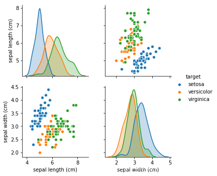
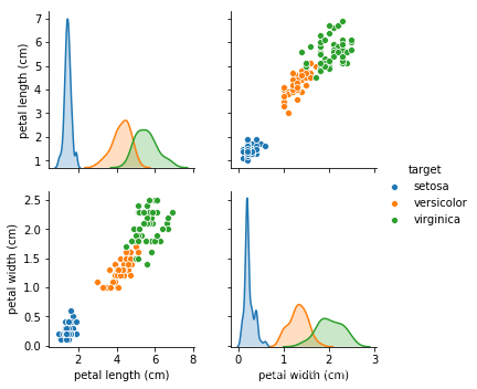
- 从以上数据能了解到此数据集内鸢尾花含有花瓣和萼片的长宽信息,画图更,清晰的展示鸢尾花的类型特征
sns.pairplot(data.iloc[:,[0,1,4]],hue='target')
sns.pairplot(data.iloc[:,2:5],hue='target')
从萼片长宽关系运行结果,可以看出不同品种的鸢尾花是各自聚集在一起的
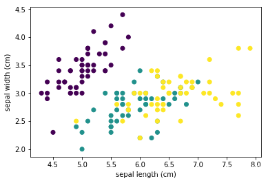
- matplotlib画散点图
plt.scatter(data1.iloc[:,0],data1.iloc[:,1],c=data1.target)
plt.xlabel('sepal length (cm)')
plt.ylabel('sepal width (cm)')
Text(0,0.5,'sepal width (cm)')
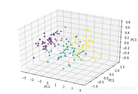
6. 机器学习降维PCA算法,把四个属性糅合在一起展现出来
from sklearn.decomposition import PCA
x_reduced = PCA(n_components=3).fit_transform(data.iloc[:,:4])
x_reduced
7.绘制成3d图形
fig=plt.figure()
ax=Axes3D(fig)
ax.scatter(x_reduced[:,0],x_reduced[:,1],x_reduced[:,2],c=data1.iloc[:,4])
ax.set_xlabel('PC1')
ax.set_ylabel('PC2')
ax.set_zlabel('PC3')
运行结果
Text(0.5,0,'PC3')
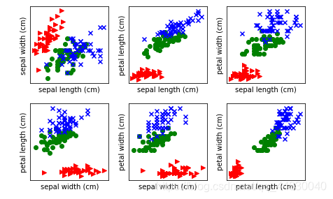
8.对数据进行处理,任意两个特征组合一个做x轴另一个做y轴进行画图
# -*- coding=utf-8 -*-
from matplotlib import pyplot as plt
from sklearn.datasets import load_iris
import numpy as np
import itertools

data = load_iris()
features = data['data']
feature_names = data['feature_names']
target = data['target']
labels = data['target_names'][data['target']]
print(data.data)
print(data.feature_names)
9.取出第二个元素,所有的两两组合
feature_names_2 = []
#排列组合
for i in range(1,len(feature_names)+1):
    iter = itertools.combinations(feature_names,i)
    feature_names_2.append(list(iter))

print(len(feature_names_2[1]))
for i in feature_names_2[1]:
    print(i)
10.在for循环里画多个子图的方法
plt.figure(1)
for i,k in enumerate(feature_names_2[1]):
    index1 = feature_names.index(k[0])
    index2 = feature_names.index(k[1])
    plt.subplot(2,3,1+i)
    for t,marker,c in zip(range(3),">ox","rgb"):
        plt.scatter(features[target==t,index1],features[target==t,index2],marker=marker,c=c)
        plt.xlabel(k[0])
        plt.ylabel(k[1])
        plt.xticks([])
        plt.yticks([])
        plt.autoscale()
        plt.tight_layout()
plt.show()
可视化效果如下
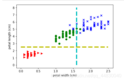
11.画水平线和垂直线
plt.figure(2)
for t,marker,c in zip(range(3),">ox","rgb"):         plt.scatter(features[target==t,3],features[target==t,2],marker=marker,c=c)
    plt.xlabel(feature_names[3])
    plt.ylabel(feature_names[2])
    # plt.xticks([])
    # plt.yticks([])
    plt.autoscale()
plt.vlines(1.6, 0, 8, colors = "c",linewidth=4,linestyles = "dashed")
plt.hlines(2.5, 0, 2.5, colors = "y",linewidth=4,linestyles = "dashed")
plt.show()
可视化效果如下