作业一
作业内容:
实现k-NN,SVM分类器,Softmax分类器和两层神经网络,实践一个简单的图像分类流程。
Softmax介绍:
SVM和Softmax分类器是最常用的两个分类器,Softmax分类器就可以理解为逻辑回归分类器面对多个分类的一般化归纳。与SVM不同,Softmax的输出(归一化的分类概率)更加直观,并且从概率上可以解释。
交叉熵损失函数:
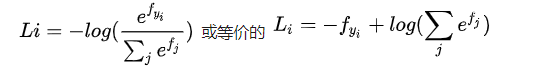
在上式中,使用fi来表示分类评分向量f中的第i个元素。和之前一样,整个数据集的损失值是数据集中所有样本数据的损失值Li的均值与正则化损失之和。
softmax 函数: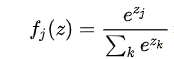
其输入值是一个向量,向量中元素为任意实数的评分值,函数对其进行压缩,输出一个向量,其中每个元素值在0到1之间,且所有元素之和为1。
不同的解释角度:
信息理论视角
在“真实”分布P和估计分布q之间的交叉熵定义如下:
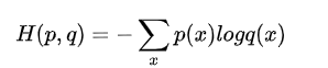
Softmax分类器所做的就是最小化在估计分类概率和“真实”分布之间的交叉熵,在这个解释中,“真实”分布就是所有概率密度都分布在正确的类别上,换句话说,交叉熵损失函数“想要”预测分布的所有概率密度都在正确分类上。
概率论解释
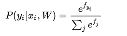
可以解释为是给定图像数据Xi,以W为参数,分配给正确分类标签yi的归一化概率。为了理解这点,请回忆一下Softmax分类器将输出向量f中的评分值解释为没有归一化的对数概率。那么以这些数值做指数函数的幂就得到了没有归一化的概率,而除法操作则对数据进行了归一化处理,使得这些概率的和为1。从概率论的角度来理解,我们就是在最小化正确分类的负对数概率,这可以看做是在进行最大似然估计(MLE)。该解释的另一个好处是,损失函数中的正则化部分可以被看做是权重矩阵W的高斯先验,这里进行的是最大后验估计(MAP)而不是最大似然估计。
数值稳定
编程实现softmax函数计算的时候因为存在指数函数,所以数值可能非常大。除以大数值可能导致数值计算的不稳定,所以学会使用归一化技巧非常重要。如果在分式的分子和分母都乘以一个常数C,并把它变换到求和之中,就能得到一个从数学上等价的公式:
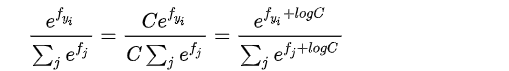
通常将C设为:
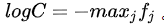
简单地说,就是应该将向量f中的数值进行平移,使得最大值为0。代码实现如下:
f = np.array([123, 456, 789]) # 例子中有3个分类,每个评分的数值都很大
p = np.exp(f) / np.sum(np.exp(f)) # 不妙:数值问题,可能导致数值爆炸

# 那么将f中的值平移到最大值为0:
f -= np.max(f) # f becomes [-666, -333, 0]
p = np.exp(f) / np.sum(np.exp(f)) # 现在OK了,将给出正确结果
SVM和Softmax的比较
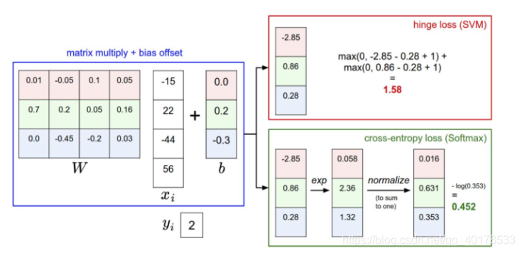
针对一个数据点,SVM和Softmax分类器的不同处理方式的例子。两个分类器都计算了同样的分值向量f(本节中是通过矩阵乘来实现)。不同之处在于对f中分值的解释:SVM分类器将它们看做是分类评分,它的损失函数鼓励正确的分类(本例中是蓝色的类别2)的分值比其他分类的分值高出至少一个边界值。Softmax分类器将这些数值看做是每个分类没有归一化的对数概率,鼓励正确分类的归一化的对数概率变高,其余的变低。SVM的最终的损失值是1.58,Softmax的最终的损失值是0.452,但要注意这两个数值没有可比性。只在给定同样数据,在同样的分类器的损失值计算中,它们才有意义。
在实际使用中,SVM和Softmax经常是相似的:通常说来,两种分类器的表现差别很小,不同的人对于哪个分类器更好有不同的看法。相对于Softmax分类器,SVM更加“局部目标化(local objective)”,这既可以看做是一个特性,也可以看做是一个劣势。考虑一个评分是[10, -2, 3]的数据,其中第一个分类是正确的。那么一个SVM会看到正确分类相较于不正确分类,已经得到了比边界值还要高的分数,它就会认为损失值是0。SVM对于数字个体的细节是不关心的:如果分数是[10, -100, -100]或者[10, 9, 9],对于SVM来说没设么不同,只要满足超过边界值等于1,那么损失值就等于0。
对于softmax分类器,情况则不同。对于[10, 9, 9]来说,计算出的损失值就远远高于[10, -100, -100]的。换句话来说,softmax分类器对于分数是永远不会满意的:正确分类总能得到更高的可能性,错误分类总能得到更低的可能性,损失值总是能够更小。但是,SVM只要边界值被满足了就满意了,不会超过限制去细微地操作具体分数。这可以被看做是SVM的一种特性。
代码
import random
import numpy as np
from cs231n.data_utils import load_CIFAR10
import matplotlib.pyplot as plt

%matplotlib inline
plt.rcParams['figure.figsize'] = (10.0, 8.0) # set default size of plots
plt.rcParams['image.interpolation'] = 'nearest'
plt.rcParams['image.cmap'] = 'gray'

%load_ext autoreload
%autoreload 2
def get_CIFAR10_data(num_training=49000, num_validation=1000, num_test=1000, num_dev=500):

    # 加载CIFAR-10 数据集
    cifar10_dir = 'cs231n/datasets/CIFAR10'

    # Cleaning up variables to prevent loading data multiple times (which may cause memory issue)
    try:
       del X_train, y_train
       del X_test, y_test
       print('Clear previously loaded data.')
    except:
       pass

    X_train, y_train, X_test, y_test = load_CIFAR10(cifar10_dir)

    # 划分数据集
    mask = list(range(num_training, num_training + num_validation))
    X_val = X_train[mask]
    y_val = y_train[mask]
    mask = list(range(num_training))
    X_train = X_train[mask]
    y_train = y_train[mask]
    mask = list(range(num_test))
    X_test = X_test[mask]
    y_test = y_test[mask]
    mask = np.random.choice(num_training, num_dev, replace=False)
    X_dev = X_train[mask]
    y_dev = y_train[mask]


    X_train = np.reshape(X_train, (X_train.shape[0], -1))
    X_val = np.reshape(X_val, (X_val.shape[0], -1))
    X_test = np.reshape(X_test, (X_test.shape[0], -1))
    X_dev = np.reshape(X_dev, (X_dev.shape[0], -1))

    # 归一化样本:减去均值化图像
    mean_image = np.mean(X_train, axis = 0)
    X_train -= mean_image
    X_val -= mean_image
    X_test -= mean_image
    X_dev -= mean_image

    # 加上偏置项
    X_train = np.hstack([X_train, np.ones((X_train.shape[0], 1))])
    X_val = np.hstack([X_val, np.ones((X_val.shape[0], 1))])
    X_test = np.hstack([X_test, np.ones((X_test.shape[0], 1))])
    X_dev = np.hstack([X_dev, np.ones((X_dev.shape[0], 1))])

    return X_train, y_train, X_val, y_val, X_test, y_test, X_dev, y_dev


X_train, y_train, X_val, y_val, X_test, y_test, X_dev, y_dev = get_CIFAR10_data()
print('Train data shape: ', X_train.shape)
print('Train labels shape: ', y_train.shape)
print('Validation data shape: ', X_val.shape)
print('Validation labels shape: ', y_val.shape)
print('Test data shape: ', X_test.shape)
print('Test labels shape: ', y_test.shape)
print('dev data shape: ', X_dev.shape)
print('dev labels shape: ', y_dev.shape)

from cs231n.classifiers.softmax import softmax_loss_naive
import time

# 随机权重W
W = np.random.randn(3073, 10) * 0.0001
loss, grad = softmax_loss_naive(W, X_dev, y_dev, 0.0)


print('loss: %f' % loss)
print('sanity check: %f' % (-np.log(0.1)))
# 梯度计算
loss, grad = softmax_loss_naive(W, X_dev, y_dev, 0.0)

# 梯度检验
from cs231n.gradient_check import grad_check_sparse
f = lambda w: softmax_loss_naive(w, X_dev, y_dev, 0.0)[0]
grad_numerical = grad_check_sparse(f, W, grad, 10)


loss, grad = softmax_loss_naive(W, X_dev, y_dev, 5e1)
f = lambda w: softmax_loss_naive(w, X_dev, y_dev, 5e1)[0]
grad_numerical = grad_check_sparse(f, W, grad, 10)
# 比较向量化和矩阵两种方式
tic = time.time()
loss_naive, grad_naive = softmax_loss_naive(W, X_dev, y_dev, 0.000005)
toc = time.time()
print('naive loss: %e computed in %fs' % (loss_naive, toc - tic))

from cs231n.classifiers.softmax import softmax_loss_vectorized
tic = time.time()
loss_vectorized, grad_vectorized = softmax_loss_vectorized(W, X_dev, y_dev, 0.000005)
toc = time.time()
print('vectorized loss: %e computed in %fs' % (loss_vectorized, toc - tic))


grad_difference = np.linalg.norm(grad_naive - grad_vectorized, ord='fro')
print('Loss difference: %f' % np.abs(loss_naive - loss_vectorized))
print('Gradient difference: %f' % grad_difference)
# 调参
from cs231n.classifiers import Softmax
results = {}
best_val = -1
best_softmax = None
learning_rates = [1e-7, 5e-7]
regularization_strengths = [2.5e4, 5e4]


for learning_rate in learning_rates:
    for regularization_strength in regularization_strengths:
        softmax = Softmax()
        loss_hist = softmax.train(X_train, y_train, learning_rate=learning_rate,
                              reg=regularization_strength, num_iters=1500, verbose=False)
        y_train_pred = softmax.predict(X_train)
        training_accuracy = np.mean(y_train == y_train_pred)
        y_val_pred = softmax.predict(X_val)
        validation_accuracy = np.mean(y_val == y_val_pred)
        results[(learning_rate, regularization_strength)] = (training_accuracy, validation_accuracy)
        if best_val < validation_accuracy:
            best_val = validation_accuracy
            best_softmax = softmax

for lr, reg in sorted(results):
    train_accuracy, val_accuracy = results[(lr, reg)]
    print('lr %e reg %e train accuracy: %f val accuracy: %f' % (
                lr, reg, train_accuracy, val_accuracy))

print('best validation accuracy achieved during cross-validation: %f' % best_val)
# 测试集
y_test_pred = best_softmax.predict(X_test)
test_accuracy = np.mean(y_test == y_test_pred)
print('softmax on raw pixels final test set accuracy: %f' % (test_accuracy, ))
# 可视化每类权重
w = best_softmax.W[:-1,:] # strip out the bias
w = w.reshape(32, 32, 3, 10)

w_min, w_max = np.min(w), np.max(w)

classes = ['plane', 'car', 'bird', 'cat', 'deer', 'dog', 'frog', 'horse', 'ship', 'truck']
for i in range(10):
    plt.subplot(2, 5, i + 1)

    wimg = 255.0 * (w[:, :, :, i].squeeze() - w_min) / (w_max - w_min)
    plt.imshow(wimg.astype('uint8'))
    plt.axis('off')
    plt.title(classes[i])
softmax.py
from builtins import range
import numpy as np
from random import shuffle
from past.builtins import xrange

def softmax_loss_naive(W, X, y, reg):
    """
    Softmax loss function, naive implementation (with loops)

    Inputs have dimension D, there are C classes, and we operate on minibatches
    of N examples.

    Inputs:
    - W: A numpy array of shape (D, C) containing weights.
    - X: A numpy array of shape (N, D) containing a minibatch of data.
    - y: A numpy array of shape (N,) containing training labels; y[i] = c means
      that X[i] has label c, where 0 <= c < C.
    - reg: (float) regularization strength

    Returns a tuple of:
    - loss as single float
    - gradient with respect to weights W; an array of same shape as W
    """
    # Initialize the loss and gradient to zero.
    loss = 0.0
    dW = np.zeros_like(W)

    #############################################################################
    # TODO: Compute the softmax loss and its gradient using explicit loops.     #
    # Store the loss in loss and the gradient in dW. If you are not careful     #
    # here, it is easy to run into numeric instability. Don't forget the        #
    # regularization!                                                           #
    #############################################################################
    # *****START OF YOUR CODE (DO NOT DELETE/MODIFY THIS LINE)*****

    num_train, dim = X.shape
    classes = W.shape[1]
    scores = X.dot(W)

    sta_scores = scores - np.max(scores, axis = 1, keepdims = True) #Numerical Stability
    exp_scores = np.exp(sta_scores)
    final_scores = exp_scores/np.sum(exp_scores, axis = 1, keepdims = True)

    for i in range(num_train):
        loss -= np.log(final_scores[i,y[i]])

    loss /= num_train
    loss += reg*np.sum(np.square(W))

    for i in range(num_train):
        for d in range(dim):
            for c in range(classes):
                dW[d, c] += (final_scores[i, c]*X[i, d])
                if c == y[i]:
                    dW[d, c] -= X[i, d]

    dW /= num_train
    dW += 2*reg*W

    # *****END OF YOUR CODE (DO NOT DELETE/MODIFY THIS LINE)*****

    return loss, dW


def softmax_loss_vectorized(W, X, y, reg):
    """
    Softmax loss function, vectorized version.

    Inputs and outputs are the same as softmax_loss_naive.
    """
    # Initialize the loss and gradient to zero.
    loss = 0.0
    dW = np.zeros_like(W)

    #############################################################################
    # TODO: Compute the softmax loss and its gradient using no explicit loops.  #
    # Store the loss in loss and the gradient in dW. If you are not careful     #
    # here, it is easy to run into numeric instability. Don't forget the        #
    # regularization!                                                           #
    #############################################################################
    # *****START OF YOUR CODE (DO NOT DELETE/MODIFY THIS LINE)*****

    num_train, dim = X.shape
    classes = W.shape[1]
    scores = X.dot(W)

    sta_scores = scores - np.max(scores, axis = 1, keepdims = True) #Numerical Stability
    exp_scores = np.exp(sta_scores)
    final_scores = exp_scores/np.sum(exp_scores, axis = 1, keepdims = True)
    loss = -np.sum(np.log(final_scores[np.arange(num_train), y]))/num_train
    loss += reg*np.sum(np.square(W))

    mask = final_scores.copy()
    mask[np.arange(num_train), y] -= 1
    dW = X.T.dot(mask)/num_train
    dW += 2*reg*W

    # *****END OF YOUR CODE (DO NOT DELETE/MODIFY THIS LINE)*****

    return loss, dW