在本作业中,你将实现循环网络,并将其应用于在微软的COCO数据库上进行图像标注。我们还会介绍TinyImageNet数据集,然后在这个数据集使用一个预训练的模型来查看图像梯度的不同应用。
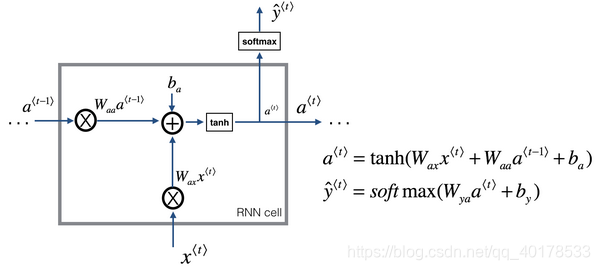
门控制单元

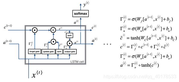
LSTM
LSTM是一个比GRU更加强大和通用的版本,这多亏了 Sepp Hochreiter和 Jurgen Schmidhuber,感谢那篇开创性的论文,它在序列模型上有着巨大影响。我感觉这篇论文是挺难读懂的,虽然我认为这篇论文在深度学习社群有着重大的影响,它深入讨论了梯度消失的理论,我感觉大部分的人学到LSTM的细节是在其他的地方,而不是这篇论文。
LSTM前向传播图:
LSTM反向传播计算:

这就是LSTM,我们什么时候应该用GRU?什么时候用LSTM?这里没有统一的准则。在深度学习的历史上,LSTM也是更早出现的,而GRU是最近才发明出来的,它可能源于Pavia在更加复杂的LSTM模型中做出的简化。研究者们在很多不同问题上尝试了这两种模型,看看在不同的问题不同的算法中哪个模型更好。
GRU的优点是这是个更加简单的模型,所以更容易创建一个更大的网络,而且它只有两个门,在计算性上也运行得更快,然后它可以扩大模型的规模。
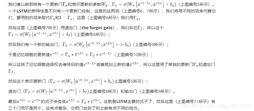
但是LSTM更加强大和灵活,因为它有三个门而不是两个。如果你想选一个使用,我认为LSTM在历史进程上是个更优先的选择,所以如果你必须选一个,我感觉今天大部分的人还是会把LSTM作为默认的选择来尝试。虽然我认为最近几年GRU获得了很多支持,而且我感觉越来越多的团队也正在使用GRU,因为它更加简单,而且还效果还不错,它更容易适应规模更加大的问题。
所以这就是LSTM,无论是GRU还是LSTM,你都可以用它们来构建捕获更加深层连接的神经网络。
使用LSTM进行图像标注
加载必要的库
import time, os, json
import numpy as np
import matplotlib.pyplot as plt

from cs231n.gradient_check import eval_numerical_gradient, eval_numerical_gradient_array
from cs231n.rnn_layers import *
from cs231n.captioning_solver import CaptioningSolver
from cs231n.classifiers.rnn import CaptioningRNN
from cs231n.coco_utils import load_coco_data, sample_coco_minibatch, decode_captions
from cs231n.image_utils import image_from_url

%matplotlib inline
plt.rcParams['figure.figsize'] = (10.0, 8.0) # set default size of plots
plt.rcParams['image.interpolation'] = 'nearest'
plt.rcParams['image.cmap'] = 'gray'

# for auto-reloading external modules
# see http://stackoverflow.com/questions/1907993/autoreload-of-modules-in-ipython
%load_ext autoreload
%autoreload 2

def rel_error(x, y):
    """ returns relative error """
    return np.max(np.abs(x - y) / (np.maximum(1e-8, np.abs(x) + np.abs(y))))
加载MS-COCO 数据集
data = load_coco_data(pca_features=True)

# Print out all the keys and values from the data dictionary
for k, v in data.items():
    if type(v) == np.ndarray:
        print(k, type(v), v.shape, v.dtype)
    else:
        print(k, type(v), len(v))
LSTM前向传播
N, D, H = 3, 4, 5
x = np.linspace(-0.4, 1.2, num=N*D).reshape(N, D)
prev_h = np.linspace(-0.3, 0.7, num=N*H).reshape(N, H)
prev_c = np.linspace(-0.4, 0.9, num=N*H).reshape(N, H)
Wx = np.linspace(-2.1, 1.3, num=4*D*H).reshape(D, 4 * H)
Wh = np.linspace(-0.7, 2.2, num=4*H*H).reshape(H, 4 * H)
b = np.linspace(0.3, 0.7, num=4*H)

next_h, next_c, cache = lstm_step_forward(x, prev_h, prev_c, Wx, Wh, b)

expected_next_h = np.asarray([
    [ 0.24635157,  0.28610883,  0.32240467,  0.35525807,  0.38474904],
    [ 0.49223563,  0.55611431,  0.61507696,  0.66844003,  0.7159181 ],
    [ 0.56735664,  0.66310127,  0.74419266,  0.80889665,  0.858299  ]])
expected_next_c = np.asarray([
    [ 0.32986176,  0.39145139,  0.451556,    0.51014116,  0.56717407],
    [ 0.66382255,  0.76674007,  0.87195994,  0.97902709,  1.08751345],
    [ 0.74192008,  0.90592151,  1.07717006,  1.25120233,  1.42395676]])

print('next_h error: ', rel_error(expected_next_h, next_h))
print('next_c error: ', rel_error(expected_next_c, next_c))
LSTM反向传播
np.random.seed(231)

N, D, H = 4, 5, 6
x = np.random.randn(N, D)
prev_h = np.random.randn(N, H)
prev_c = np.random.randn(N, H)
Wx = np.random.randn(D, 4 * H)
Wh = np.random.randn(H, 4 * H)
b = np.random.randn(4 * H)

next_h, next_c, cache = lstm_step_forward(x, prev_h, prev_c, Wx, Wh, b)

dnext_h = np.random.randn(*next_h.shape)
dnext_c = np.random.randn(*next_c.shape)

fx_h = lambda x: lstm_step_forward(x, prev_h, prev_c, Wx, Wh, b)[0]
fh_h = lambda h: lstm_step_forward(x, prev_h, prev_c, Wx, Wh, b)[0]
fc_h = lambda c: lstm_step_forward(x, prev_h, prev_c, Wx, Wh, b)[0]
fWx_h = lambda Wx: lstm_step_forward(x, prev_h, prev_c, Wx, Wh, b)[0]
fWh_h = lambda Wh: lstm_step_forward(x, prev_h, prev_c, Wx, Wh, b)[0]
fb_h = lambda b: lstm_step_forward(x, prev_h, prev_c, Wx, Wh, b)[0]

fx_c = lambda x: lstm_step_forward(x, prev_h, prev_c, Wx, Wh, b)[1]
fh_c = lambda h: lstm_step_forward(x, prev_h, prev_c, Wx, Wh, b)[1]
fc_c = lambda c: lstm_step_forward(x, prev_h, prev_c, Wx, Wh, b)[1]
fWx_c = lambda Wx: lstm_step_forward(x, prev_h, prev_c, Wx, Wh, b)[1]
fWh_c = lambda Wh: lstm_step_forward(x, prev_h, prev_c, Wx, Wh, b)[1]
fb_c = lambda b: lstm_step_forward(x, prev_h, prev_c, Wx, Wh, b)[1]

num_grad = eval_numerical_gradient_array

dx_num = num_grad(fx_h, x, dnext_h) + num_grad(fx_c, x, dnext_c)
dh_num = num_grad(fh_h, prev_h, dnext_h) + num_grad(fh_c, prev_h, dnext_c)
dc_num = num_grad(fc_h, prev_c, dnext_h) + num_grad(fc_c, prev_c, dnext_c)
dWx_num = num_grad(fWx_h, Wx, dnext_h) + num_grad(fWx_c, Wx, dnext_c)
dWh_num = num_grad(fWh_h, Wh, dnext_h) + num_grad(fWh_c, Wh, dnext_c)
db_num = num_grad(fb_h, b, dnext_h) + num_grad(fb_c, b, dnext_c)

dx, dh, dc, dWx, dWh, db = lstm_step_backward(dnext_h, dnext_c, cache)

print('dx error: ', rel_error(dx_num, dx))
print('dh error: ', rel_error(dh_num, dh))
print('dc error: ', rel_error(dc_num, dc))
print('dWx error: ', rel_error(dWx_num, dWx))
print('dWh error: ', rel_error(dWh_num, dWh))
print('db error: ', rel_error(db_num, db))
整个时间步上的LSTM的前向传播和反向传播
N, D, H, T = 2, 5, 4, 3
x = np.linspace(-0.4, 0.6, num=N*T*D).reshape(N, T, D)
h0 = np.linspace(-0.4, 0.8, num=N*H).reshape(N, H)
Wx = np.linspace(-0.2, 0.9, num=4*D*H).reshape(D, 4 * H)
Wh = np.linspace(-0.3, 0.6, num=4*H*H).reshape(H, 4 * H)
b = np.linspace(0.2, 0.7, num=4*H)

h, cache = lstm_forward(x, h0, Wx, Wh, b)

expected_h = np.asarray([
 [[ 0.01764008,  0.01823233,  0.01882671,  0.0194232 ],
  [ 0.11287491,  0.12146228,  0.13018446,  0.13902939],
  [ 0.31358768,  0.33338627,  0.35304453,  0.37250975]],
 [[ 0.45767879,  0.4761092,   0.4936887,   0.51041945],
  [ 0.6704845,   0.69350089,  0.71486014,  0.7346449 ],
  [ 0.81733511,  0.83677871,  0.85403753,  0.86935314]]])

print('h error: ', rel_error(expected_h, h))

from cs231n.rnn_layers import lstm_forward, lstm_backward
np.random.seed(231)

N, D, T, H = 2, 3, 10, 6

x = np.random.randn(N, T, D)
h0 = np.random.randn(N, H)
Wx = np.random.randn(D, 4 * H)
Wh = np.random.randn(H, 4 * H)
b = np.random.randn(4 * H)

out, cache = lstm_forward(x, h0, Wx, Wh, b)

dout = np.random.randn(*out.shape)

dx, dh0, dWx, dWh, db = lstm_backward(dout, cache)

fx = lambda x: lstm_forward(x, h0, Wx, Wh, b)[0]
fh0 = lambda h0: lstm_forward(x, h0, Wx, Wh, b)[0]
fWx = lambda Wx: lstm_forward(x, h0, Wx, Wh, b)[0]
fWh = lambda Wh: lstm_forward(x, h0, Wx, Wh, b)[0]
fb = lambda b: lstm_forward(x, h0, Wx, Wh, b)[0]

dx_num = eval_numerical_gradient_array(fx, x, dout)
dh0_num = eval_numerical_gradient_array(fh0, h0, dout)
dWx_num = eval_numerical_gradient_array(fWx, Wx, dout)
dWh_num = eval_numerical_gradient_array(fWh, Wh, dout)
db_num = eval_numerical_gradient_array(fb, b, dout)

print('dx error: ', rel_error(dx_num, dx))
print('dh0 error: ', rel_error(dh0_num, dh0))
print('dWx error: ', rel_error(dWx_num, dWx))
print('dWh error: ', rel_error(dWh_num, dWh))
print('db error: ', rel_error(db_num, db))
LSTM模型
N, D, W, H = 10, 20, 30, 40
word_to_idx = {'<NULL>': 0, 'cat': 2, 'dog': 3}
V = len(word_to_idx)
T = 13

model = CaptioningRNN(word_to_idx,
          input_dim=D,
          wordvec_dim=W,
          hidden_dim=H,
          cell_type='lstm',
          dtype=np.float64)

# Set all model parameters to fixed values
for k, v in model.params.items():
  model.params[k] = np.linspace(-1.4, 1.3, num=v.size).reshape(*v.shape)

features = np.linspace(-0.5, 1.7, num=N*D).reshape(N, D)
captions = (np.arange(N * T) % V).reshape(N, T)

loss, grads = model.loss(features, captions)
expected_loss = 9.82445935443

print('loss: ', loss)
print('expected loss: ', expected_loss)
print('difference: ', abs(loss - expected_loss))
训练
np.random.seed(231)

small_data = load_coco_data(max_train=50)

small_lstm_model = CaptioningRNN(
          cell_type='lstm',
          word_to_idx=data['word_to_idx'],
          input_dim=data['train_features'].shape[1],
          hidden_dim=512,
          wordvec_dim=256,
          dtype=np.float32,
        )

small_lstm_solver = CaptioningSolver(small_lstm_model, small_data,
           update_rule='adam',
           num_epochs=50,
           batch_size=25,
           optim_config={
             'learning_rate': 5e-3,
           },
           lr_decay=0.995,
           verbose=True, print_every=10,
         )

small_lstm_solver.train()

# Plot the training losses
plt.plot(small_lstm_solver.loss_history)
plt.xlabel('Iteration')
plt.ylabel('Loss')
plt.title('Training loss history')
plt.show()
测试
for split in ['train', 'val']:
    minibatch = sample_coco_minibatch(small_data, split=split, batch_size=2)
    gt_captions, features, urls = minibatch
    gt_captions = decode_captions(gt_captions, data['idx_to_word'])

    sample_captions = small_lstm_model.sample(features)
    sample_captions = decode_captions(sample_captions, data['idx_to_word'])

    for gt_caption, sample_caption, url in zip(gt_captions, sample_captions, urls):
        plt.imshow(image_from_url(url))
        plt.title('%s\n%s\nGT:%s' % (split, sample_caption, gt_caption))
        plt.axis('off')
        plt.show()