作业一
作业内容:
实现k-NN,SVM分类器,Softmax分类器和两层神经网络,实践一个简单的图像分类流程。
激活函数类型:

上图左边是Sigmoid非线性函数,将实数压缩到[0,1]之间。右边是tanh函数,将实数压缩到[-1,1]。
然而现在sigmoid函数已经不太受欢迎,实际很少使用了,这是因为它有***两个主要缺点***:
- Sigmoid函数饱和使梯度消失
- Sigmoid函数的输出不是零中心的
和sigmoid神经元一样,tanh函数也存在饱和问题,但是和sigmoid神经元不同的是,它的输出是零中心的。现在大多使用tanh
——————————————————————————————

左边是ReLU(校正线性单元:Rectified Linear Unit)激活函数,当X=0时函数值为0。当X>0时函数的斜率为1。右边是从 Krizhevsky等的论文中截取的图表,指明使用ReLU比使用tanh的收敛快6倍。
使用ReLU有以下一些优缺点:
优点 - 相较于sigmoid和tanh函数,ReLU对于随机梯度下降的收敛有巨大的加速作用
- sigmoid和tanh神经元含有指数运算等耗费计算资源的操作,而ReLU可以简单地通过对一个矩阵进行阈值计算得到
缺点 - 在训练的时候,ReLU单元比较脆弱并且可能“死掉”。举例来说,当一个很大的梯度流过ReLU的神经元的时候,可能会导致梯度更新到一种特别的状态,在这种状态下神经元将无法被其他任何数据点再次激活。如果这种情况发生,那么从此所以流过这个神经元的梯度将都变成0。也就是说,这个ReLU单元在训练中将不可逆转的死亡,因为这导致了数据多样化的丢失。
以上就是一些常用的神经元及其激活函数。
——————————————————————————————
Leaky ReLU。Leaky ReLU是为解决“ReLU死亡”问题的尝试。ReLU中当x<0时,函数值为0。而Leaky ReLU则是给出一个很小的负数梯度值,比如0.01。
Maxout。一些其他类型的单元被提了出来,Maxout是对ReLU和leaky ReLU的一般化归纳,它的函数是:

eLU和Leaky ReLU都是这个公式的特殊情况(比如ReLU就是当W1,b1=0的时候)。这样Maxout神经元就拥有ReLU单元的所有优点(线性操作和不饱和),而没有它的缺点(死亡的ReLU单元)。然而和ReLU对比,它每个神经元的参数数量增加了一倍,这就导致整体参数的数量激增。
——————————————————————————————
最后需要注意一点:在同一个网络中混合使用不同类型的神经元是非常少见的,虽然没有什么根本性问题来禁止这样做。
数据预处理
- 均值减法:是预处理最常用的形式。它对数据中每个独立特征减去平均值,从几何上可以理解为在每个维度上都将数据云的中心都迁移到原点.
- 归一化:是指将数据的所有维度都归一化,使其数值范围都近似相等。有两种常用方法可以实现归一化。

一般数据预处理流程:左边:原始的2维输入数据。中间:在每个维度上都减去平均值后得到零中心化数据,现在数据云是以原点为中心的。右边:每个维度都除以其标准差来调整其数值范围。红色的线指出了数据各维度的数值范围,在中间的零中心化数据的数值范围不同,但在右边归一化数据中数值范围相同。 - PCA:是另一种预处理形式。在这种处理中,先对数据进行零中心化处理,然后计算协方差矩阵,它展示了数据中的相关性结构.
- 白化:白化操作的输入是特征基准上的数据,然后对每个维度除以其特征值来对数值范围进行归一化。该变换的几何解释是:如果数据服从多变量的高斯分布,那么经过白化后,数据的分布将会是一个均值为零,且协方差相等的矩阵。确定夸大的噪声。
权重初始化
- 错误:全零初始化。
让我们从应该避免的错误开始。在训练完毕后,虽然不知道网络中每个权重的最终值应该是多少,但如果数据经过了恰当的归一化的话,就可以假设所有权重数值中大约一半为正数,一半为负数。这样,一个听起来蛮合理的想法就是把这些权重的初始值都设为0吧,因为在期望上来说0是最合理的猜测。这个做法错误的!因为如果网络中的每个神经元都计算出同样的输出,然后它们就会在反向传播中计算出同样的梯度,从而进行同样的参数更新。换句话说,如果权重被初始化为同样的值,神经元之间就失去了不对称性的源头。 - 小随机数初始化:因此,权重初始值要非常接近0又不能等于0。解决方法就是将权重初始化为很小的数值,以此来打破对称性。
- 稀疏初始化:另一个处理非标定方差的方法是将所有权重矩阵设为0,但是为了打破对称性,每个神经元都同下一层固定数目的神经元随机连接(其权重数值由一个小的高斯分布生成)。一个比较典型的连接数目是10个。
- 偏置(biases)的初始化:通常将偏置初始化为0,这是因为随机小数值权重矩阵已经打破了对称性。对于ReLU非线性激活函数,有研究人员喜欢使用如0.01这样的小数值常量作为所有偏置的初始值,这是因为他们认为这样做能让所有的ReLU单元一开始就激活,这样就能保存并传播一些梯度。然而,这样做是不是总是能提高算法性能并不清楚(有时候实验结果反而显示性能更差),所以通常还是使用0来初始化偏置参数。
批量归一化
批量归一化是loffe和Szegedy提出的方法,该方法减轻了如何合理初始化神经网络这个棘手问题带来的头痛:,其做法是让激活数据在训练开始前通过一个网络,网络处理数据使其服从标准高斯分布。因为归一化是一个简单可求导的操作,所以上述思路是可行的。在实现层面,应用这个技巧通常意味着全连接层与激活函数之间添加一个BatchNorm层。对于这个技巧本节不会展开讲,因为上面的参考文献中已经讲得很清楚了,需要知道的是在神经网络中使用批量归一化已经变得非常常见。在实践中,使用了批量归一化的网络对于不好的初始值有更强的鲁棒性。最后一句话总结:批量归一化可以理解为在网络的每一层之前都做预处理,只是这种操作以另一种方式与网络集成在了一起。
正则化 Regularization
- L2正则化可能是最常用的正则化方法了。可以通过惩罚目标函数中所有参数的平方将其实现。即对于网络中的每个权重W
- L1正则化是另一个相对常用的正则化方法
- 最大范式约束另一种形式的正则化是给每个神经元中权重向量的量级设定上限,并使用投影梯度下降来确保这一约束。
- 随机失活是一个简单又极其有效的正则化方法。与L1正则化,L2正则化和最大范式约束等方法互为补充。在训练的时候,随机失活的实现方法是让神经元以超参数P的概率被激活或者被设置为0。
梯度检查
理论上将进行梯度检查很简单,就是简单地把解析梯度和数值计算梯度进行比较。然而从实际操作层面上来说,这个过程更加复杂且容易出错。下面是一些提示、技巧和需要仔细注意的事情:
使用中心化公式。在使用有限差值近似来计算数值梯度的时候,常见的公式是
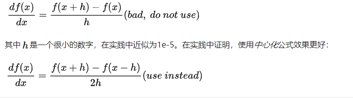
该公式在检查梯度的每个维度的时候,会要求计算两次损失函数(所以计算资源的耗费也是两倍),但是梯度的近似值会准确很多。
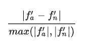
使用相对误差来比较:
比较数值梯度和解析梯度的细节有哪些?如何得知此两者不匹配?你可能会倾向于监测它们的差的绝对值或者差的平方值,然后定义该值如果超过某个规定阈值,就判断梯度实现失败。然而该思路是有问题的。想想,假设这个差值是1e-4,如果两个梯度值在1.0左右,这个差值看起来就很合适,可以认为两个梯度是匹配的。然而如果梯度值是1e-5或者更低,那么1e-4就是非常大的差距,梯度实现肯定就是失败的了。因此,使用相对误差总是更合适一些:
- 相对误差>1e-2:通常就意味着梯度可能出错。
- 1e-2>相对误差>1e-4:要对这个值感到不舒服才行。
- 1e-4>相对误差:这个值的相对误差对于有不可导点的目标函数是OK的。但如果目标函数中没有kink(使用tanh和softmax),那么相对误差值还是太高。
- 1e-7或者更小:好结果,可以高兴一把了。
要知道的是网络的深度越深,相对误差就越高。所以如果你是在对一个10层网络的输入数据做梯度检查,那么1e-2的相对误差值可能就OK了,因为误差一直在累积。相反,如果一个可微函数的相对误差值是1e-2,那么通常说明梯度实现不正确。
使用双精度
一个常见的错误是使用单精度浮点数来进行梯度检查。这样会导致即使梯度实现正确,相对误差值也会很高(比如1e-2)。在我的经验而言,出现过使用单精度浮点数时相对误差为1e-2,换成双精度浮点数时就降低为1e-8的情况。
学习之前:合理性检查的提示与技巧
在进行费时费力的最优化之前,最好进行一些合理性检查:
- ***寻找特定情况的正确损失值。***在使用小参数进行初始化时,确保得到的损失值与期望一致。最好先单独检查数据损失(让正则化强度为0)。例如,对于一个跑CIFAR-10的Softmax分类器,一般期望它的初始损失值是2.302,这是因为初始时预计每个类别的概率是0.1(因为有10个类别),然后Softmax损失值正确分类的负对数概率:-ln(0.1)=2.302。对于Weston Watkins SVM,假设所有的边界都被越过(因为所有的分值都近似为零),所以损失值是9(因为对于每个错误分类,边界值是1)。如果没看到这些损失值,那么初始化中就可能有问题。
- 第二个合理性检查:提高正则化强度时导致损失值变大。
- 对小数据子集过拟合:最后也是最重要的一步,在整个数据集进行训练之前,尝试在一个很小的数据集上进行训练(比如20个数据),然后确保能到达0的损失值。进行这个实验的时候,最好让正则化强度为0,不然它会阻止得到0的损失。除非能通过这一个正常性检查,不然进行整个数据集训练是没有意义的。但是注意,能对小数据集进行过拟合并不代表万事大吉,依然有可能存在不正确的实现。比如,因为某些错误,数据点的特征是随机的,这样算法也可能对小数据进行过拟合,但是在整个数据集上跑算法的时候,就没有任何泛化能力。
损失函数
训练期间第一个要跟踪的数值就是损失值,它在前向传播时对每个独立的批数据进行计算。下图展示的是随着损失值随时间的变化,尤其是曲线形状会给出关于学习率设置的情况:

左图展示了不同的学习率的效果。过低的学习率导致算法的改善是线性的。高一些的学习率会看起来呈几何指数下降,更高的学习率会让损失值很快下降,但是接着就停在一个不好的损失值上(绿线)。这是因为最优化的“能量”太大,参数在混沌中随机震荡,不能最优化到一个很好的点上。右图显示了一个典型的随时间变化的损失函数值,在CIFAR-10数据集上面训练了一个小的网络,这个损失函数值曲线看起来比较合理(虽然可能学习率有点小,但是很难说),而且指出了批数据的数量可能有点太小(因为损失值的噪音很大)。
——————————————————————————————
训练集和验证集准确率
在训练分类器的时候,需要跟踪的第二重要的数值是验证集和训练集的准确率。这个图表能够展现知道模型过拟合的程度:
 在训练集准确率和验证集准确率中间的空隙指明了模型过拟合的程度。在图中,蓝色的验证集曲线显示相较于训练集,验证集的准确率低了很多,这就说明模型有很强的过拟合。遇到这种情况,就应该增大正则化强度(更强的L2权重惩罚,更多的随机失活等)或收集更多的数据。另一种可能就是验证集曲线和训练集曲线如影随形,这种情况说明你的模型容量还不够大:应该通过增加参数数量让模型容量更大些。
每层的激活数据及梯度分布
一个不正确的初始化可能让学习过程变慢,甚至彻底停止。还好,这个问题可以比较简单地诊断出来。其中一个方法是输出网络中所有层的激活数据和梯度分布的柱状图。直观地说,就是如果看到任何奇怪的分布情况,那都不是好兆头。比如,对于使用tanh的神经元,我们应该看到激活数据的值在整个[-1,1]区间中都有分布。如果看到神经元的输出全部是0,或者全都饱和了往-1和1上跑,那肯定就是有问题了。
第一层可视化
 将神经网络第一层的权重可视化的例子。左图中的特征充满了噪音,这暗示了网络可能出现了问题:网络没有收敛,学习率设置不恰当,正则化惩罚的权重过低。右图的特征不错,平滑,干净而且种类繁多,说明训练过程进行良好。
代码
import numpy as np
import matplotlib.pyplot as plt

from cs231n.classifiers.neural_net import TwoLayerNet

%matplotlib inline
plt.rcParams['figure.figsize'] = (10.0, 8.0) # set default size of plots
plt.rcParams['image.interpolation'] = 'nearest'
plt.rcParams['image.cmap'] = 'gray'

%load_ext autoreload
%autoreload 2
# 矢量间的相对误差计算
def rel_error(x, y):
    """ returns relative error """
    return np.max(np.abs(x - y) / (np.maximum(1e-8, np.abs(x) + np.abs(y))))
input_size = 4
hidden_size = 10
num_classes = 3
# 样本 5*4
num_inputs = 5

def init_toy_model():
    np.random.seed(0)
    return TwoLayerNet(input_size, hidden_size, num_classes, std=1e-1)

def init_toy_data():
    np.random.seed(1)
    X = 10 * np.random.randn(num_inputs, input_size)
    y = np.array([0, 1, 2, 2, 1])
    return X, y

net = init_toy_model()
X, y = init_toy_data()
scores = net.loss(X)
print('Your scores:')
print(scores)
print()
print('correct scores:')
correct_scores = np.asarray([
  [-0.81233741, -1.27654624, -0.70335995],
  [-0.17129677, -1.18803311, -0.47310444],
  [-0.51590475, -1.01354314, -0.8504215 ],
  [-0.15419291, -0.48629638, -0.52901952],
  [-0.00618733, -0.12435261, -0.15226949]])
print(correct_scores)
print()

# 差距应该 < 1e-7
print('Difference between your scores and correct scores:')
print(np.sum(np.abs(scores - correct_scores)))
# 加入正则化
loss, _ = net.loss(X, y, reg=0.05)
correct_loss = 1.30378789133

# s差距< 1e-12
print('Difference between your loss and correct loss:')
print(np.sum(np.abs(loss - correct_loss)))
from cs231n.gradient_check import eval_numerical_gradient

# 使用梯度检测来检验反向传播的梯度,W1,W2,b1和b2的每个分析梯度应小于1e-8
loss, grads = net.loss(X, y, reg=0.05)
for param_name in grads:
    f = lambda W: net.loss(X, y, reg=0.05)[0]
    param_grad_num = eval_numerical_gradient(f, net.params[param_name], verbose=False)
    print('%s max relative error: %e' % (param_name, rel_error(param_grad_num, grads[param_name])))
net = init_toy_model()
stats = net.train(X, y, X, y,
            learning_rate=1e-1, reg=5e-6,
            num_iters=100, verbose=False)

print('Final training loss: ', stats['loss_history'][-1])

# 画出损失曲线
plt.plot(stats['loss_history'])
plt.xlabel('iteration')
plt.ylabel('training loss')
plt.title('Training Loss history')
plt.show()
from cs231n.data_utils import load_CIFAR10

def get_CIFAR10_data(num_training=49000, num_validation=1000, num_test=1000):
    # 划分数据集
    # Load the raw CIFAR-10 data
    cifar10_dir = 'cs231n/datasets/CIFAR10'

    # Cleaning up variables to prevent loading data multiple times (which may cause memory issue)
    try:
       del X_train, y_train
       del X_test, y_test
       print('Clear previously loaded data.')
    except:
       pass

    X_train, y_train, X_test, y_test = load_CIFAR10(cifar10_dir)

    # Subsample the data
    mask = list(range(num_training, num_training + num_validation))
    X_val = X_train[mask]
    y_val = y_train[mask]
    mask = list(range(num_training))
    X_train = X_train[mask]
    y_train = y_train[mask]
    mask = list(range(num_test))
    X_test = X_test[mask]
    y_test = y_test[mask]

    # Normalize the data: subtract the mean image
    mean_image = np.mean(X_train, axis=0)
    X_train -= mean_image
    X_val -= mean_image
    X_test -= mean_image

    # Reshape data to rows
    X_train = X_train.reshape(num_training, -1)
    X_val = X_val.reshape(num_validation, -1)
    X_test = X_test.reshape(num_test, -1)

    return X_train, y_train, X_val, y_val, X_test, y_test


# Invoke the above function to get our data.
X_train, y_train, X_val, y_val, X_test, y_test = get_CIFAR10_data()
print('Train data shape: ', X_train.shape)
print('Train labels shape: ', y_train.shape)
print('Validation data shape: ', X_val.shape)
print('Validation labels shape: ', y_val.shape)
print('Test data shape: ', X_test.shape)
print('Test labels shape: ', y_test.shape)
input_size = 32 * 32 * 3
hidden_size = 50
num_classes = 10
net = TwoLayerNet(input_size, hidden_size, num_classes)

# Train the network
stats = net.train(X_train, y_train, X_val, y_val,
            num_iters=1000, batch_size=200,
            learning_rate=1e-4, learning_rate_decay=0.95,
            reg=0.25, verbose=True)

# Predict on the validation set
val_acc = (net.predict(X_val) == y_val).mean()
print('Validation accuracy: ', val_acc)
# 绘制损失函数,训练、验证集上的准确率
plt.subplot(2, 1, 1)
plt.plot(stats['loss_history'])
plt.title('Loss history')
plt.xlabel('Iteration')
plt.ylabel('Loss')

plt.subplot(2, 1, 2)
plt.plot(stats['train_acc_history'], label='train')
plt.plot(stats['val_acc_history'], label='val')
plt.title('Classification accuracy history')
plt.xlabel('Epoch')
plt.ylabel('Classification accuracy')
plt.legend()
plt.show()
from cs231n.vis_utils import visualize_grid

# 可视化网络权重

def show_net_weights(net):
    W1 = net.params['W1']
    W1 = W1.reshape(32, 32, 3, -1).transpose(3, 0, 1, 2)
    plt.imshow(visualize_grid(W1, padding=3).astype('uint8'))
    plt.gca().axis('off')
    plt.show()

show_net_weights(net)
best_net = None # store the best model into this
# 调参
results = {}
best_val = -1
learning_rates = [1e-3, 5e-4]
regularization_strengths = [0.25, 0.5]

input_size = 32 * 32 * 3
hidden_size = 100
num_classes = 10
net = TwoLayerNet(input_size, hidden_size, num_classes)

for learning_rate in learning_rates:
    for regularization_strength in regularization_strengths:
        net = TwoLayerNet(input_size, hidden_size, num_classes)
        loss_hist = net.train(X_train, y_train, X_val, y_val,
            num_iters=1000, batch_size=200,
            learning_rate=learning_rate, learning_rate_decay=0.95,
            reg=regularization_strength, verbose=False)
        y_train_pred = net.predict(X_train)
        training_accuracy = np.mean(y_train == y_train_pred)
        y_val_pred = net.predict(X_val)
        validation_accuracy = np.mean(y_val == y_val_pred)
        results[(learning_rate, regularization_strength)] = (training_accuracy, validation_accuracy)
        if best_val < validation_accuracy:
            best_val = validation_accuracy
            best_net = net
# 测试集上的精度
test_acc = (best_net.predict(X_test) == y_test).mean()
print('Test accuracy: ', test_acc)
neural_net.py
from __future__ import print_function

from builtins import range
from builtins import object
import numpy as np
import matplotlib.pyplot as plt
from past.builtins import xrange

class TwoLayerNet(object):
    """
    A two-layer fully-connected neural network. The net has an input dimension of
    N, a hidden layer dimension of H, and performs classification over C classes.
    We train the network with a softmax loss function and L2 regularization on the
    weight matrices. The network uses a ReLU nonlinearity after the first fully
    connected layer.

    In other words, the network has the following architecture:

    input - fully connected layer - ReLU - fully connected layer - softmax

    The outputs of the second fully-connected layer are the scores for each class.
    """

    def __init__(self, input_size, hidden_size, output_size, std=1e-4):
        """
        Initialize the model. Weights are initialized to small random values and
        biases are initialized to zero. Weights and biases are stored in the
        variable self.params, which is a dictionary with the following keys:

        W1: First layer weights; has shape (D, H)
        b1: First layer biases; has shape (H,)
        W2: Second layer weights; has shape (H, C)
        b2: Second layer biases; has shape (C,)

        Inputs:
        - input_size: The dimension D of the input data.
        - hidden_size: The number of neurons H in the hidden layer.
        - output_size: The number of classes C.
        """
        self.params = {}
        self.params['W1'] = std * np.random.randn(input_size, hidden_size)
        self.params['b1'] = np.zeros(hidden_size)
        self.params['W2'] = std * np.random.randn(hidden_size, output_size)
        self.params['b2'] = np.zeros(output_size)

    def loss(self, X, y=None, reg=0.0):
        """
        Compute the loss and gradients for a two layer fully connected neural
        network.

        Inputs:
        - X: Input data of shape (N, D). Each X[i] is a training sample.
        - y: Vector of training labels. y[i] is the label for X[i], and each y[i] is
          an integer in the range 0 <= y[i] < C. This parameter is optional; if it
          is not passed then we only return scores, and if it is passed then we
          instead return the loss and gradients.
        - reg: Regularization strength.

        Returns:
        If y is None, return a matrix scores of shape (N, C) where scores[i, c] is
        the score for class c on input X[i].

        If y is not None, instead return a tuple of:
        - loss: Loss (data loss and regularization loss) for this batch of training
          samples.
        - grads: Dictionary mapping parameter names to gradients of those parameters
          with respect to the loss function; has the same keys as self.params.
        """
        # Unpack variables from the params dictionary
        W1, b1 = self.params['W1'], self.params['b1']
        W2, b2 = self.params['W2'], self.params['b2']
        N, D = X.shape

        # Compute the forward pass
        scores = None
        #############################################################################
        # TODO: Perform the forward pass, computing the class scores for the input. #
        # Store the result in the scores variable, which should be an array of      #
        # shape (N, C).                                                             #
        #############################################################################
        # *****START OF YOUR CODE (DO NOT DELETE/MODIFY THIS LINE)*****

        z1 = X.dot(W1)+b1
        a1 = np.maximum(0, z1)
        scores = a1.dot(W2)+b2

        # *****END OF YOUR CODE (DO NOT DELETE/MODIFY THIS LINE)*****

        # If the targets are not given then jump out, we're done
        if y is None:
            return scores

        # Compute the loss
        loss = None
        #############################################################################
        # TODO: Finish the forward pass, and compute the loss. This should include  #
        # both the data loss and L2 regularization for W1 and W2. Store the result  #
        # in the variable loss, which should be a scalar. Use the Softmax           #
        # classifier loss.                                                          #
        #############################################################################
        # *****START OF YOUR CODE (DO NOT DELETE/MODIFY THIS LINE)*****

        exp_scores = np.exp(scores-np.max(scores, axis = 1, keepdims = True))
        final_scores = exp_scores/np.sum(exp_scores, axis=1, keepdims = True)
        loss = np.sum(-np.log(final_scores[np.arange(N),y]))/N
        loss += reg*np.sum(np.square(W1))
        loss += reg*np.sum(np.square(W2))

        # *****END OF YOUR CODE (DO NOT DELETE/MODIFY THIS LINE)*****

        # Backward pass: compute gradients
        grads = {}
        #############################################################################
        # TODO: Compute the backward pass, computing the derivatives of the weights #
        # and biases. Store the results in the grads dictionary. For example,       #
        # grads['W1'] should store the gradient on W1, and be a matrix of same size #
        #############################################################################
        # *****START OF YOUR CODE (DO NOT DELETE/MODIFY THIS LINE)*****

        dexp_scores = np.ones(exp_scores.shape)/np.sum(exp_scores, axis=1, keepdims = True)
        dexp_scores[np.arange(N), y] -= 1/exp_scores[np.arange(N), y]
        dexp_scores /= N
        dscores = exp_scores*dexp_scores
        db2 = np.sum(dscores,axis=0)
        dW2 = a1.T.dot(dscores)
        da1 = dscores.dot(W2.T)
        dz1 = da1
        dz1[z1 <= 0] = 0
        db1 = np.sum(dz1, axis=0)
        dW1 = X.T.dot(dz1)

        dW1 += 2*reg*W1
        dW2 += 2*reg*W2
        grads['W1'] = dW1
        grads['b1'] = db1
        grads['W2'] = dW2
        grads['b2'] = db2

        # *****END OF YOUR CODE (DO NOT DELETE/MODIFY THIS LINE)*****

        return loss, grads

    def train(self, X, y, X_val, y_val,
              learning_rate=1e-3, learning_rate_decay=0.95,
              reg=5e-6, num_iters=100,
              batch_size=200, verbose=False):
        """
        Train this neural network using stochastic gradient descent.

        Inputs:
        - X: A numpy array of shape (N, D) giving training data.
        - y: A numpy array f shape (N,) giving training labels; y[i] = c means that
          X[i] has label c, where 0 <= c < C.
        - X_val: A numpy array of shape (N_val, D) giving validation data.
        - y_val: A numpy array of shape (N_val,) giving validation labels.
        - learning_rate: Scalar giving learning rate for optimization.
        - learning_rate_decay: Scalar giving factor used to decay the learning rate
          after each epoch.
        - reg: Scalar giving regularization strength.
        - num_iters: Number of steps to take when optimizing.
        - batch_size: Number of training examples to use per step.
        - verbose: boolean; if true print progress during optimization.
        """
        num_train = X.shape[0]
        iterations_per_epoch = max(num_train / batch_size, 1)

        # Use SGD to optimize the parameters in self.model
        loss_history = []
        train_acc_history = []
        val_acc_history = []

        for it in range(num_iters):
            X_batch = None
            y_batch = None

            #########################################################################
            # TODO: Create a random minibatch of training data and labels, storing  #
            # them in X_batch and y_batch respectively.                             #
            #########################################################################
            # *****START OF YOUR CODE (DO NOT DELETE/MODIFY THIS LINE)*****

            incides = np.random.choice(num_train,batch_size,replace = True)
            X_batch = X[incides]
            y_batch = y[incides]

            # *****END OF YOUR CODE (DO NOT DELETE/MODIFY THIS LINE)*****

            # Compute loss and gradients using the current minibatch
            loss, grads = self.loss(X_batch, y=y_batch, reg=reg)
            loss_history.append(loss)

            #########################################################################
            # TODO: Use the gradients in the grads dictionary to update the         #
            # parameters of the network (stored in the dictionary self.params)      #
            # using stochastic gradient descent. You'll need to use the gradients   #
            # stored in the grads dictionary defined above.                         #
            #########################################################################
            # *****START OF YOUR CODE (DO NOT DELETE/MODIFY THIS LINE)*****

            self.params['W1'] -= learning_rate*grads['W1']
            self.params['W2'] -= learning_rate*grads['W2']
            self.params['b1'] -= learning_rate*grads['b1']
            self.params['b2'] -= learning_rate*grads['b2']

            # *****END OF YOUR CODE (DO NOT DELETE/MODIFY THIS LINE)*****

            if verbose and it % 100 == 0:
                print('iteration %d / %d: loss %f' % (it, num_iters, loss))

            # Every epoch, check train and val accuracy and decay learning rate.
            if it % iterations_per_epoch == 0:
                # Check accuracy
                train_acc = (self.predict(X_batch) == y_batch).mean()
                val_acc = (self.predict(X_val) == y_val).mean()
                train_acc_history.append(train_acc)
                val_acc_history.append(val_acc)

                # Decay learning rate
                learning_rate *= learning_rate_decay

        return {
          'loss_history': loss_history,
          'train_acc_history': train_acc_history,
          'val_acc_history': val_acc_history,
        }

    def predict(self, X):
        """
        Use the trained weights of this two-layer network to predict labels for
        data points. For each data point we predict scores for each of the C
        classes, and assign each data point to the class with the highest score.

        Inputs:
        - X: A numpy array of shape (N, D) giving N D-dimensional data points to
          classify.

        Returns:
        - y_pred: A numpy array of shape (N,) giving predicted labels for each of
          the elements of X. For all i, y_pred[i] = c means that X[i] is predicted
          to have class c, where 0 <= c < C.
        """
        y_pred = None

        ###########################################################################
        # TODO: Implement this function; it should be VERY simple!                #
        ###########################################################################
        # *****START OF YOUR CODE (DO NOT DELETE/MODIFY THIS LINE)*****

        scores = np.maximum(X.dot(self.params['W1']) + self.params['b1'], 0).dot(self.params['W2']) + self.params['b2']
        y_pred = np.argsort(scores,axis = 1)[:,-1]

        # *****END OF YOUR CODE (DO NOT DELETE/MODIFY THIS LINE)*****

        return y_pred