##读取图片并将图片中的像素点数据标准化
import os
import struct
import numpy as np
def load_mnist(path, kind='train'):
"""Load MNIST data from `path`"""
labels_path = os.path.join(path,
'%s-labels-idx1-ubyte' % kind)
images_path = os.path.join(path,'%s-images-idx3-ubyte' % kind)
with open(labels_path, 'rb') as lbpath:

#其中>表示big-endian,I表示无符号整数

magic, n = struct.unpack('>II',lbpath.read(8))
labels = np.fromfile(lbpath,
dtype=np.uint8)
with open(images_path, 'rb') as imgpath:
magic, num, rows, cols = struct.unpack(">IIII",
imgpath.read(16))
images = np.fromfile(imgpath,
dtype=np.uint8).reshape(
len(labels), 784)

#标准化像素值到-1到1

images = ((images / 255.) - .5) * 2
return images, labels
##展示数据的维数
X_train, y_train = load_mnist('', kind='train')
   print('Rows: %d, columns: %d'% (X_train.shape[0], X_train.shape[1]))
X_test, y_test = load_mnist('', kind='t10k')
print('Rows: %d, columns: %d'% (X_test.shape[0], X_test.shape[1]))

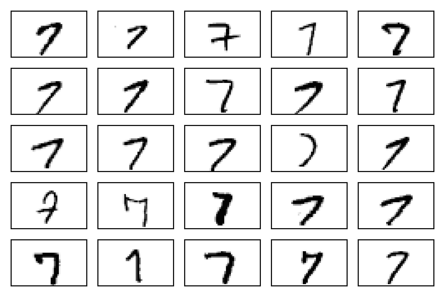
##展示示例特征矩阵中的784像素向量重新整形后的数字0-9原始的28×28图像,不同的手写字体的不同
fig, ax = plt.subplots(nrows=5,
... ncols=5,
... sharex=True,
... sharey=True)
ax = ax.flatten()
for i in range(25):
... img = X_train[y_train == 7][i].reshape(28, 28)
... ax[i].imshow(img, cmap='Greys')
ax[0].set_xticks([])
ax[0].set_yticks([])
plt.tight_layout()
plt.show()
#train the MLP using 55,000 samples from the already shuffled MNIST training dataset
#and use the remaining 5,000 samples for validation during training
import numpy as np
import sys
class NeuralNetMLP(object):
    """ Feedforward neural network / Multi-layer perceptron classifier.

    Parameters
    ------------
    n_hidden : int (default: 30)
        Number of hidden units.
    l2 : float (default: 0.)
        Lambda value for L2-regularization.
        No regularization if l2=0. (default)
    epochs : int (default: 100)
        Number of passes over the training set.
    eta : float (default: 0.001)
        Learning rate.
    shuffle : bool (default: True)
        Shuffles training data every epoch if True to prevent circles.
    minibatch_size : int (default: 1)
        Number of training samples per minibatch.
    seed : int (default: None)
        Random seed for initalizing weights and shuffling.

    Attributes
    -----------
    eval_ : dict
      Dictionary collecting the cost, training accuracy,
      and validation accuracy for each epoch during training.

    """
    def __init__(self, n_hidden=30,
                 l2=0., epochs=100, eta=0.001,
                 shuffle=True, minibatch_size=1, seed=None):

        self.random = np.random.RandomState(seed)
        self.n_hidden = n_hidden
        self.l2 = l2
        self.epochs = epochs
        self.eta = eta
        self.shuffle = shuffle
        self.minibatch_size = minibatch_size

    def _onehot(self, y, n_classes):
        """Encode labels into one-hot representation

        Parameters
        ------------
        y : array, shape = [n_samples]
            Target values.

        Returns
        -----------
        onehot : array, shape = (n_samples, n_labels)

        """
        onehot = np.zeros((n_classes, y.shape[0]))
        for idx, val in enumerate(y):
            onehot[val, idx] = 1.
        return onehot.T

    def _sigmoid(self, z):
        """Compute logistic function (sigmoid)"""
        return 1. / (1. + np.exp(-np.clip(z, -250, 250)))

    def _forward(self, X):
        """Compute forward propagation step"""

        # step 1: net input of hidden layer
        # [n_samples, n_features] dot [n_features, n_hidden]
        # -> [n_samples, n_hidden]
        z_h = np.dot(X, self.w_h) + self.b_h

        # step 2: activation of hidden layer
        a_h = self._sigmoid(z_h)

        # step 3: net input of output layer
        # [n_samples, n_hidden] dot [n_hidden, n_classlabels]
        # -> [n_samples, n_classlabels]

        z_out = np.dot(a_h, self.w_out) + self.b_out

        # step 4: activation output layer
        a_out = self._sigmoid(z_out)

        return z_h, a_h, z_out, a_out

    def _compute_cost(self, y_enc, output):
        """Compute cost function.

        Parameters
        ----------
        y_enc : array, shape = (n_samples, n_labels)
            one-hot encoded class labels.
        output : array, shape = [n_samples, n_output_units]
            Activation of the output layer (forward propagation)

        Returns
        ---------
        cost : float
            Regularized cost

        """
        L2_term = (self.l2 *
                   (np.sum(self.w_h ** 2.) +
                    np.sum(self.w_out ** 2.)))

        term1 = -y_enc * (np.log(output))
        term2 = (1. - y_enc) * np.log(1. - output)
        cost = np.sum(term1 - term2) + L2_term

        # If you are applying this cost function to other
        # datasets where activation
        # values maybe become more extreme (closer to zero or 1)
        # you may encounter "ZeroDivisionError"s due to numerical
        # instabilities in Python & NumPy for the current implementation.
        # I.e., the code tries to evaluate log(0), which is undefined.
        # To address this issue, you could add a small constant to the
        # activation values that are passed to the log function.
        #
        # For example:
        #
        # term1 = -y_enc * (np.log(output + 1e-5))
        # term2 = (1. - y_enc) * np.log(1. - output + 1e-5)

        return cost

    def predict(self, X):
        """Predict class labels

        Parameters
        -----------
        X : array, shape = [n_samples, n_features]
            Input layer with original features.

        Returns:
        ----------
        y_pred : array, shape = [n_samples]
            Predicted class labels.

        """
        z_h, a_h, z_out, a_out = self._forward(X)
        y_pred = np.argmax(z_out, axis=1)
        return y_pred

    def fit(self, X_train, y_train, X_valid, y_valid):
        """ Learn weights from training data.

        Parameters
        -----------
        X_train : array, shape = [n_samples, n_features]
            Input layer with original features.
        y_train : array, shape = [n_samples]
            Target class labels.
        X_valid : array, shape = [n_samples, n_features]
            Sample features for validation during training
        y_valid : array, shape = [n_samples]
            Sample labels for validation during training

        Returns:
        ----------
        self

        """
        n_output = np.unique(y_train).shape[0]  # number of class labels
        n_features = X_train.shape[1]

        ########################
        # Weight initialization
        ########################

        # weights for input -> hidden
        self.b_h = np.zeros(self.n_hidden)
        self.w_h = self.random.normal(loc=0.0, scale=0.1,
                                      size=(n_features, self.n_hidden))

        # weights for hidden -> output
        self.b_out = np.zeros(n_output)
        self.w_out = self.random.normal(loc=0.0, scale=0.1,
                                        size=(self.n_hidden, n_output))

        epoch_strlen = len(str(self.epochs))  # for progress formatting
        self.eval_ = {'cost': [], 'train_acc': [], 'valid_acc': []}

        y_train_enc = self._onehot(y_train, n_output)

        # iterate over training epochs
        for i in range(self.epochs):

            # iterate over minibatches
            indices = np.arange(X_train.shape[0])

            if self.shuffle:
                self.random.shuffle(indices)

            for start_idx in range(0, indices.shape[0] - self.minibatch_size +
                                   1, self.minibatch_size):
                batch_idx = indices[start_idx:start_idx + self.minibatch_size]

                # forward propagation
                z_h, a_h, z_out, a_out = self._forward(X_train[batch_idx])

                ##################
                # Backpropagation
                ##################

                # [n_samples, n_classlabels]
                sigma_out = a_out - y_train_enc[batch_idx]

                # [n_samples, n_hidden]
                sigmoid_derivative_h = a_h * (1. - a_h)

                # [n_samples, n_classlabels] dot [n_classlabels, n_hidden]
                # -> [n_samples, n_hidden]
                sigma_h = (np.dot(sigma_out, self.w_out.T) *
                           sigmoid_derivative_h)

                # [n_features, n_samples] dot [n_samples, n_hidden]
                # -> [n_features, n_hidden]
                grad_w_h = np.dot(X_train[batch_idx].T, sigma_h)
                grad_b_h = np.sum(sigma_h, axis=0)

                # [n_hidden, n_samples] dot [n_samples, n_classlabels]
                # -> [n_hidden, n_classlabels]
                grad_w_out = np.dot(a_h.T, sigma_out)
                grad_b_out = np.sum(sigma_out, axis=0)

                # Regularization and weight updates
                delta_w_h = (grad_w_h + self.l2*self.w_h)
                delta_b_h = grad_b_h  # bias is not regularized
                self.w_h -= self.eta * delta_w_h
                self.b_h -= self.eta * delta_b_h

                delta_w_out = (grad_w_out + self.l2*self.w_out)
                delta_b_out = grad_b_out  # bias is not regularized
                self.w_out -= self.eta * delta_w_out
                self.b_out -= self.eta * delta_b_out

            #############
            # Evaluation
            #############

            # Evaluation after each epoch during training
            z_h, a_h, z_out, a_out = self._forward(X_train)
            cost = self._compute_cost(y_enc=y_train_enc,
                                      output=a_out)

            y_train_pred = self.predict(X_train)
            y_valid_pred = self.predict(X_valid)

            train_acc = ((np.sum(y_train == y_train_pred)).astype(np.float) /
                         X_train.shape[0])
            valid_acc = ((np.sum(y_valid == y_valid_pred)).astype(np.float) /
                         X_valid.shape[0])

            sys.stderr.write('\r%0*d/%d | Cost: %.2f '
                             '| Train/Valid Acc.: %.2f%%/%.2f%% ' %
                             (epoch_strlen, i+1, self.epochs, cost,
                              train_acc*100, valid_acc*100))
            sys.stderr.flush()

            self.eval_['cost'].append(cost)
            self.eval_['train_acc'].append(train_acc)
            self.eval_['valid_acc'].append(valid_acc)

        return self
nn.fit(X_train=X_train[:55000],y_train=y_train[:55000],

X_valid=X_train[55000:],y_valid=y_train[55000:])

import matplotlib.pyplot as plt
plt.plot(range(nn.epochs), nn.eval_['cost'])
 plt.ylabel('Cost')
plt.xlabel('Epochs')
plt.show()
 对图像进行分析可知,当ecochs=100时,cost逐渐开始收敛,坡度减缓,到145,200时仍然逐渐减小。
plt.plot(range(nn.epochs), nn.eval_['train_acc'],label='training')
plt.plot(range(nn.epochs), nn.eval_['valid_acc'],label='validation', linestyle='--')
plt.ylabel('Accuracy')
plt.xlabel('Epochs')
plt.legend()
plt.show()

该图显示训练和验证准确度之间的差距增加我们训练网络的Epochs越来越多。
大约在第50个Epochs,训练和验证准确度值相等,然后网络开始过拟和训练数据。
y_test_pred = nn.predict(X_test)
acc = (np.sum(y_test == y_test_pred).astype(np.float) / X_test.shape[0])
print('Training accuracy: %.2f%%' % (acc * 100))

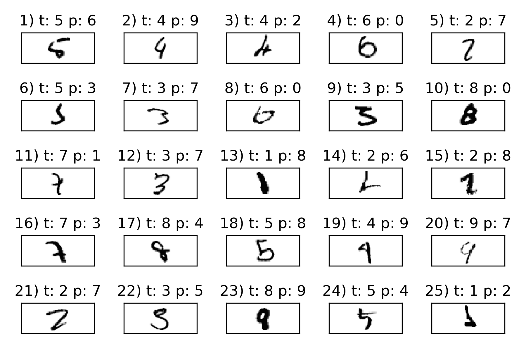
#查看25个被错误分类的例子
miscl_img = X_test[y_test != y_test_pred][:25]
correct_lab = y_test[y_test != y_test_pred][:25]
miscl_lab= y_test_pred[y_test != y_test_pred][:25]
fig, ax = plt.subplots(nrows=5,
ncols=5,sharex=True, sharey=True,)
ax = ax.flatten()
for i in range(25):
... img = miscl_img[i].reshape(28, 28)
... ax[i].imshow(img,
... cmap='Greys',
... interpolation='nearest')
... ax[i].set_title('%d) t: %d p: %d'
... % (i+1, correct_lab[i], miscl_lab[i]))
ax[0].set_xticks([])
ax[0].set_yticks([])
plt.tight_layout()
plt.show()
引入tensorflow,对上述的算法进行改进:在这里我们将用双曲线代替隐藏层中的逻辑单元切线激活函数(tanh),用softmax替换输出中的逻辑函数,并添加一个额外的隐藏层。
import tensorflow as tf
n_features = X_train_centered.shape[1]
n_classes = 10
random_seed = 123
np.random.seed(random_seed)
g = tf.Graph()
with g.as_default():
tf.set_random_seed(random_seed)
tf_x = tf.placeholder(dtype=tf.float32,
shape=(None, n_features),
name='tf_x')
tf_y = tf.placeholder(dtype=tf.int32,
shape=None, name='tf_y')
y_onehot = tf.one_hot(indices=tf_y, depth=n_classes)
h1 = tf.layers.dense(inputs=tf_x, units=50,
activation=tf.tanh,
name='layer1')
h2 = tf.layers.dense(inputs=h1, units=50,
activation=tf.tanh,
name='layer2')
logits = tf.layers.dense(inputs=h2,
units=10,
activation=None,
name='layer3')
predictions = {
'classes' : tf.argmax(logits, axis=1,
name='predicted_classes'),
'probabilities' : tf.nn.softmax(logits,
name='softmax_tensor')
}
## define cost function and optimizer:
with g.as_default():
cost = tf.losses.softmax_cross_entropy(
onehot_labels=y_onehot, logits=logits)
optimizer = tf.train.GradientDescentOptimizer(
learning_rate=0.001)
train_op = optimizer.minimize(
loss=cost)
init_op = tf.global_variables_initializer()
#return a generator batches of data
def create_batch_generator(X, y, batch_size=128, shuffle=False):
X_copy = np.array(X)
y_copy = np.array(y)
if shuffle:
data = np.column_stack((X_copy, y_copy))
np.random.shuffle(data)
X_copy = data[:, :-1]
y_copy = data[:, -1].astype(int)
for i in range(0, X.shape[0], batch_size):
yield (X_copy[i:i+batch_size, :], y_copy[i:i+batch_size])>>> ## create a session to launch the graph
>>> sess = tf.Session(graph=g)
>>> ## run the variable initialization operator
>>> sess.run(init_op)
>>>
>>> ## 50 epochs of training:
>>> for epoch in range(50):
... training_costs = []
... batch_generator = create_batch_generator(
... X_train_centered, y_train,
... batch_size=64, shuffle=True)
... for batch_X, batch_y in batch_generator:
... ## prepare a dict to feed data to our network:
... feed = {tf_x:batch_X, tf_y:batch_y}
... _, batch_cost = sess.run([train_op, cost],
feed_dict=feed)
... training_costs.append(batch_cost)
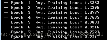
... print(' -- Epoch %2d '
... 'Avg. Training Loss: %.4f' % (
... epoch+1, np.mean(training_costs)
... ))
>>> ## do prediction on the test set:
>>> feed = {tf_x : X_test_centered}
>>> y_pred = sess.run(predictions['classes'],
... feed_dict=feed)
>>>
>>> print('Test Accuracy: %.2f%%' % (

... 100*np.sum(y_pred == y_test)/y_test.shape[0]))

使用karas生成神经网络
#set the random seed for NumPy and TensorFlow to get consistent results

>>> import tensorflow as tf
>>> import tensorflow.contrib.keras as keras
>>> np.random.seed(123)

>>> tf.set_random_seed(123)

#convert the class labels (integers 0-9) into the one-hot format

>>> y_train_onehot = keras.utils.to_categorical(y_train)
>>> print('First 3 labels: ', y_train[:3])
First 3 labels: [5 0 4]

>>> print('\nFirst 3 labels (one-hot):\n', y_train_onehot[:3])
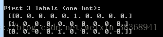
#initialize a new model using

model = keras.models.Sequential()

#add there layers ,first two layers each have 50 hidden units with tanh activation function and last layer has 10 layers #for 10 class labels and use softmax to give the probability of each class.

model.add(
keras.layers.Dense(
units=50,
input_dim=X_train_centered.shape[1],
kernel_initializer='glorot_uniform',
bias_initializer='zeros',
activation='tanh'))
model.add(
keras.layers.Dense(
units=50,
input_dim=50,
kernel_initializer='glorot_uniform',
bias_initializer='zeros',
activation='tanh'))
model.add(
keras.layers.Dense(
units=y_train_onehot.shape[1],
input_dim=50,
kernel_initializer='glorot_uniform',
bias_initializer='zeros',
activation='softmax'))
sgd_optimizer = keras.optimizers.SGD(
lr=0.001, decay=1e-7, momentum=.9)

#设置随机梯度下降

model.compile(optimizer=sgd_optimizer,
loss='categorical_crossentropy')

#train the MLP over 50 epochs,by setting verbose=1,we can follow the
#optimization of the cost function during training

>>> history = model.fit(X_train_centered, y_train_onehot,
... batch_size=64, epochs=50,
... verbose=1,

... validation_split=0.1)

#print the model accuracy on training and test sets

>>> y_train_pred = model.predict_classes(X_train_centered,

... verbose=0)
>>> correct_preds = np.sum(y_train == y_train_pred, axis=0)
>>> train_acc = correct_preds / y_train.shape[0]
>>>
>>> print('First 3 predictions: ', y_train_pred[:3])
First 3 predictions: [5 0 4]
>>>

>>> print('Training accuracy: %.2f%%' % (train_acc * 100))

>>> y_test_pred = model.predict_classes(X_test_centered,
... verbose=0)
>>> correct_preds = np.sum(y_test == y_test_pred, axis=0)
>>> test_acc = correct_preds / y_test.shape[0]

>>> print('Test accuracy: %.2f%%' % (test_acc * 100))
