Python Machine Learning

Chapter 3:A Tour of Machine Learning Classifiers Using Scikit-learn

3.1：Training a perceptron via scikit-learn

from sklearn import datasets
import numpy as np
iris = datasets.load_iris()
X = iris.data[:, [2, 3]]
y = iris.target
np.unique(y)

from sklearn.cross_validation import train_test_split
#从150个样本中随机抽取30%的样本作为test_data
X_train, X_test, y_train, y_test = train_test_split(X,y,test_size=0.3, random_state=0)

#数据归一化
#StandardScaler estimated the parameters μ(sample mean) and (standard deviation)
#(x - mean)/(standard deviation)
from sklearn.preprocessing import StandardScaler
sc = StandardScaler()
sc.fit(X_train)
X_train_std = sc.transform(X_train)
X_test_std = sc.transform(X_test)

#Perceptron分类
#eta0 is equivalent to the learning rate
from sklearn.linear_model import Perceptron
ppn = Perceptron(n_iter=40, eta0=0.1, random_state=0)
ppn.fit(X_train_std, y_train)

y_pred = ppn.predict(X_test_std)
#y_test != y_pred
'''
array([False, False, False, False, False, False, False, False, False,
       False,  True, False, False, False, False, False, False, False,
       False, False, False, False, False, False, False, False, False,
       False,  True, False, False, False, False, False, False,  True,
       False,  True, False, False, False, False, False, False, False])

'''
print('Misclassified samples: %d' % (y_test != y_pred).sum())
#Misclassified samples: 4
#Thus, the misclassification error on the test dataset is 0.089 or 8.9 percent (4/45)

#the metrics module:performance metrics
from sklearn.metrics import accuracy_score
print('Accuracy: %.2f' % accuracy_score(y_test, y_pred))
#Accuracy:0.91

#plot_decision_regions:visualize how well it separates the different flower samples
from matplotlib.colors import ListedColormap
import matplotlib.pyplot as plt

def plot_decision_regions(X, y, classifier, test_idx=None, resolution=0.02):
      #setup marker generator and color map
      markers = ('s', 'x', 'o', '^', 'v')
      colors = ('red', 'blue', 'lightgreen', 'black', 'cyan')
      cmap = ListedColormap(colors[:len(np.unique(y))])

      # plot the decision surface
      x1_min, x1_max = X[:, 0].min() -1, X[:, 0].max() + 1
      x2_min, x2_max = X[:, 1].min() -1, X[:, 1].max() + 1
      xx1, xx2 = np.meshgrid(np.arange(x1_min, x1_max, resolution), np.arange(x2_min, x2_max, resolution))
      Z = classifier.predict(np.array([xx1.ravel(), xx2.ravel()]).T)
      Z = Z.reshape(xx1.shape)
      plt.contourf(xx1, xx2, Z, alpha=0.4, cmap=cmap)
      plt.xlim(xx1.min(), xx1.max())
      plt.ylim(xx2.min(), xx2.max())

      # plot all samples
      for idx, c1 in enumerate(np.unique(y)):
            print idx,c1
            plt.scatter(x=X[y == c1, 0], y=X[y == c1, 1], alpha=0.8, c=cmap(idx),marker=markers[idx],label=c1)

      #highlight test samples
      if test_idx :
            X_test, y_test = X[test_idx, :], y[test_idx]

            #把 corlor 设置为空，通过edgecolors来控制颜色
            plt.scatter(X_test[:, 0],X_test[:, 1], color='',edgecolors='black', alpha=1.0, linewidths=2, marker='o',s=150, label='test set')
            

X_combined_std = np.vstack((X_train_std, X_test_std))
y_combined = np.hstack((y_train, y_test))
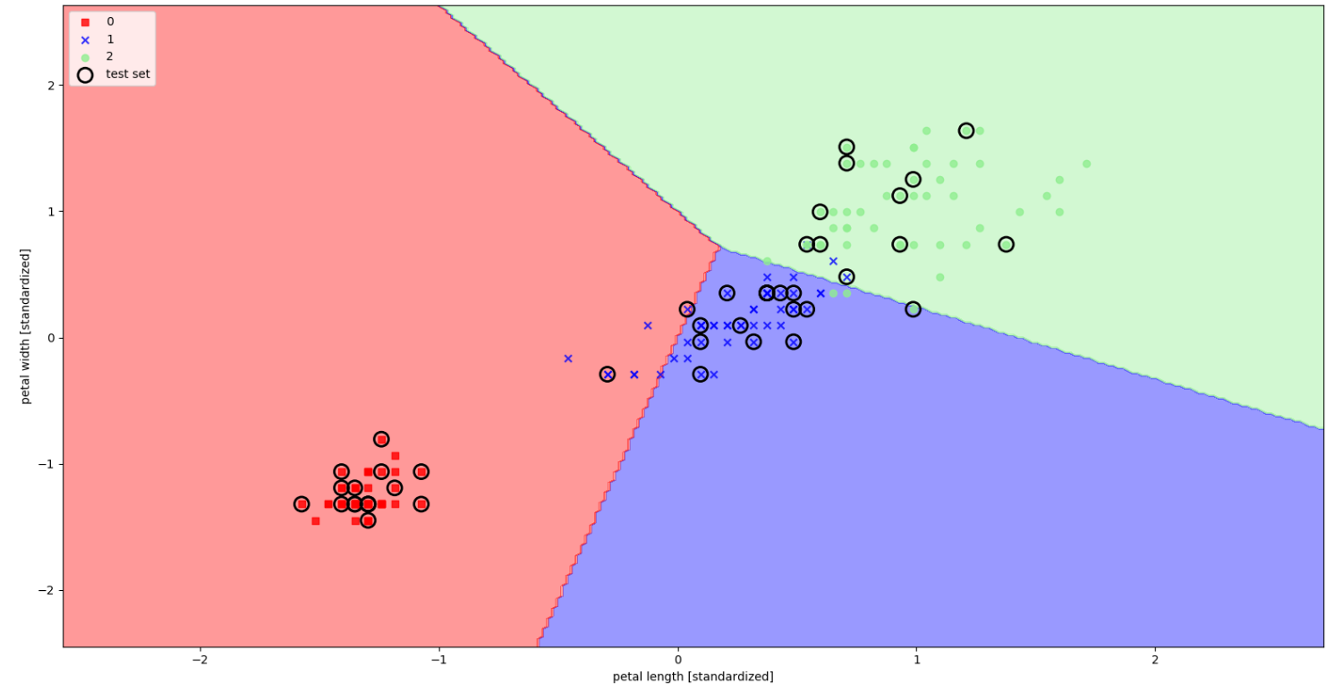
plot_decision_regions(X=X_combined_std, y=y_combined, classifier=ppn, test_idx=range(105,150))
plt.xlabel('petal length [standardized]')
plt.ylabel('petal width [standardized]')
plt.legend(loc='upper left')
plt.show()