- 为什么要引入正则化?
在做线性回归或者逻辑回归的时候,会遇到过拟合问题,即,在训练集上的error很小,但是在测试集上的偏差却很大。因此,引入正则化项,防止过拟合。保证在测试集上获得和在训练集上相同的效果。
例如:对于线性回归,不同幂次的方程如下

通过训练得到的结果如下:

明显,对于低次方程,容易产生欠拟合,而对于高次方程,容易产生过拟合现象。
因此,我们引入正则化项:

其他的正则化因子

- 关于线性回归的正则化
(1)首先,绘制数据图像:
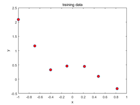
我们可以看到,只有7个数据点,因此,很容易过拟合,(训练数据集越大,越不容易过拟合)。
(2)我们用一个五次的多项式做线性回归:
![]()
之所以是线性回归,是因为对于每一个x的不同幂次,它们是线性组合的。对于初始的x,它是一个一维的特征,因此,我们将x重新构造,得到一个六维的向量。
m=length(y);
x=[ones(m,1),x,x.^2,x.^3,x.^4,x.^5];
如上实现,那么对于x的每一个维度,它们都是线性无关的,h(x)是它们的线性组合,因此,此时问题是一个多维线性回归问题。
(3)损失函数

其中λ是正则化参数。
(4)采用正规方程方式求解

注意:λ后的矩阵,θ0不参与计算,即不对θ0进行惩罚。
对于不同的参数λ,如果过大,则会把所有的参数都最小化了,导致模型编程常数θ0
即造成欠拟合。
(5)计算方法:
lambda=1;
Lambda=lambda.*eye(6);
Lambda(1)=0;
theta=(x'*x+Lambda)\x'*y
figure;
x_=(minx:0.01:maxx)';
x_1=[ones(size(x_)),x_,x_.^2,x_.^3,x_.^4,x_.^5]
hold on
plot(x0, y0, 'o', 'MarkerFacecolor', 'r', 'MarkerSize', 8);
plot(x_,x_1*theta,'--b','LineWidth',2);
legend({'data','5-th line'})
title('\lambda=1')
xlabel('x')
ylabel('y')
hold off


其中λ取0,1,10.结果如下:
计算结果如下:
Theta(λ=0) = 6×1 0.4725 0.6814 -1.3801 -5.9777 2.4417 4.7371Theta(λ=1) = 6×1 0.3976 -0.4207 0.1296 -0.3975 0.1753 -0.3394Theta(λ=10) = 6×1 0.5205 -0.1825 0.0606 -0.1482 0.0743 -0.1280
我们可以看出,当λ=0时,曲线很好的拟合了数据点,但是也明显产生了过拟合;而当λ=1时,数据点相对均匀地分布在曲线的两侧,而λ=10时,欠拟合现象明显。
- 关于逻辑回归的正则化
- 绘制原始数据

其中,‘+’表示正例,‘o’表示反例。
绘制方法如下:
pos = find(y); neg = find(y == 0);
plot (x(pos,1),x(pos,2),'+')
hold on
plot (x(neg,1),x(neg,2),'o')
- 预测函数与x的转化

注意:x是一个二维的向量,我们此处将x转化为一个高维的向量,同时,最高次数为6.特征映射函数如下:
function out = map_feature(feat1, feat2)
degree = 6;
out = ones(size(feat1(:,1)));
for i = 1:degree
for j = 0:i
out(:, end+1) = (feat1.^(i-j)).*(feat2.^j);
end
end

正则化后的损失函数

参数θ的更新规则,其中H是Hessian矩阵,另一个参数为J的梯度。

- 迭代求解
-
[m, n] = size(x);
theta = zeros(n, 1);
g =@(z)(1.0 ./ (1.0 + exp(-z)));
% disp(theta)
lambda=0
iteration=20
J = zeros(iteration, 1);
for i=1:iteration
z = x*theta;% x:117x28 theta 28x1
h = g(z) ;% sigmoid h
% Calculate J (for testing convergence)
J(i) =-(1/m)*sum(y.*log(h)+(1-y).*log(1-h))+ ...
(lambda/(2*m))*norm(theta(2:end))^2; %不包括theta(0)
%norm求的是向量theta的欧几里德范数
% Calculate gradient and hessian.
G = (lambda/m).*theta; G(1) = 0; % gradient
L = (lambda/m).*eye(n); L(1) = 0;% Hessian
grad = ((1/m).*x' * (h-y)) + G;
H = ((1/m).*x'*diag(h)*diag(1-h)*x) + L;
% Here is the actual update
theta = theta - H\grad;
end
计算出θ的值,然后绘制决策边界,可视化展示计算结果。
- 结果展示
-
其中λ的取值同样为0,1,10;
注意,采用MATLAB中的contour函数通过等高线的方式进行绘制,同时,在取值连线的时候注意要对u,v做同样的处理,如下:
% Define the ranges of the grid
u = linspace(-1, 1.5, 200);
v = linspace(-1, 1.5, 200);
% Initialize space for the values to be plotted
z = zeros(length(u), length(v));
% Evaluate z = theta*x over the grid
for i = 1:length(u)
for j = 1:length(v)
% Notice the order of j, i here!
z(j,i) = map_feature(u(i), v(j))*theta;
end
end
绘制图像结果如下:

-

-

-
同样,我们可以看到对于λ=0,过拟合,λ=10,欠拟合。
附录 源代码
附录:程序源代码
1.	线性回归+正则化
2.	clc,clear
3.	x=load("ex5Linx.dat");
4.	y=load("ex5Liny.dat");
5.	x0=x,y0=y
6.	figure;
7.	plot(x, y, 'o', 'MarkerFacecolor', 'r', 'MarkerSize', 8);
8.	title('training data')
9.	xlabel('x')
10.	ylabel('y')
11.	minx=min(x);
12.	maxx=max(x);
13.	m=length(y);
14.	x=[ones(m,1),x,x.^2,x.^3,x.^4,x.^5];
15.	disp(size(x(1,:)))   %1x6
16.	theta=zeros(size(x(1,:)))
17.	lambda=0;
18.	Lambda=lambda.*eye(6);
19.	Lambda(1)=0;
20.	theta=(x'*x+Lambda)\x'*y
21.	figure;
22.	x_=(minx:0.01:maxx)';
23.	x_1=[ones(size(x_)),x_,x_.^2,x_.^3,x_.^4,x_.^5]
24.	hold on
25.	plot(x0, y0, 'o', 'MarkerFacecolor', 'r', 'MarkerSize', 8);
26.	plot(x_,x_1*theta,'--b','LineWidth',2);
27.	legend({'data','5-th line'})
28.	title('\lambda=0')
29.	xlabel('x')
30.	ylabel('y')
31.	hold off
32.	lambda=1;
33.	Lambda=lambda.*eye(6);
34.	Lambda(1)=0;
35.	theta=(x'*x+Lambda)\x'*y
36.	figure;
37.	x_=(minx:0.01:maxx)';
38.	x_1=[ones(size(x_)),x_,x_.^2,x_.^3,x_.^4,x_.^5]
39.	hold on
40.	plot(x0, y0, 'o', 'MarkerFacecolor', 'r', 'MarkerSize', 8);
41.	plot(x_,x_1*theta,'--b','LineWidth',2);
42.	legend({'data','5-th line'})
43.	title('\lambda=1')
44.	xlabel('x')
45.	ylabel('y')
46.	hold off
47.	lambda=10;
48.	Lambda=lambda.*eye(6);
49.	Lambda(1)=0;
50.	theta=(x'*x+Lambda)\x'*y
51.	figure;
52.	x_=(minx:0.01:maxx)';
53.	x_1=[ones(size(x_)),x_,x_.^2,x_.^3,x_.^4,x_.^5]
54.	hold on
55.	plot(x0, y0, 'o', 'MarkerFacecolor', 'r', 'MarkerSize', 8);
56.	plot(x_,x_1*theta,'--b','LineWidth',2);
57.	legend({'data','5-th line'})
58.	title('\lambda=10')
59.	xlabel('x')
60.	ylabel('y')
61.	hold off

2.	逻辑回归+正则化
1.	clc,clear;
2.	x = load ('ex5Logx.dat') ;
3.	y = load ('ex5Logy.dat') ;
4.	x0=x
5.	y0=y
6.	figure
7.	% Find the i n d i c e s f or th e 2 c l a s s e s
8.	pos = find(y); neg = find(y == 0);
9.	plot (x(pos,1),x(pos,2),'+')
10.	hold on
11.	plot (x(neg,1),x(neg,2),'o')
12.	u=x(:,1)
13.	v=x(:,2)
14.	x = map_feature (u,v)
15.	[m, n] = size(x);
16.	theta = zeros(n, 1);
17.	g =@(z)(1.0 ./ (1.0 + exp(-z)));
18.	% disp(theta)
19.	lambda=0
20.	iteration=20
21.	J = zeros(iteration, 1);
22.	for i=1:iteration
23.	    z = x*theta;%  x:117x28 theta 28x1
24.	    h = g(z) ;%  sigmoid   h
25.
26.	    % Calculate J (for testing convergence)
27.	    J(i) =-(1/m)*sum(y.*log(h)+(1-y).*log(1-h))+ ...
28.	    (lambda/(2*m))*norm(theta(2:end))^2; %不包括theta(0)
29.	    %norm求的是向量theta的欧几里德范数
30.
31.	    % Calculate gradient and hessian.
32.	    G = (lambda/m).*theta; G(1) = 0; % gradient
33.	    L = (lambda/m).*eye(n); L(1) = 0;% Hessian
34.
35.	    grad = ((1/m).*x' * (h-y)) + G;
36.	    H = ((1/m).*x'*diag(h)*diag(1-h)*x) + L;
37.
38.	    % Here is the actual update
39.	    theta = theta - H\grad;
40.
41.	end
42.	% Define the ranges of the grid
43.	u = linspace(-1, 1.5, 200);
44.	v = linspace(-1, 1.5, 200);
45.
46.	% Initialize space for the values to be plotted
47.	z = zeros(length(u), length(v));
48.
49.	% Evaluate z = theta*x over the grid
50.	for i = 1:length(u)
51.	    for j = 1:length(v)
52.	        % Notice the order of j, i here!
53.	        z(j,i) = map_feature(u(i), v(j))*theta;
54.	    end
55.	end
56.	% Because of the way that contour plotting works
57.	% in Matlab, we need to transpose z, or
58.	% else the axis orientation will be flipped!
59.	z = z'
60.	% Plot z = 0 by specifying the range [0, 0]
61.	contour(u,v,z,[0,0], 'LineWidth', 2)
62.	xlim([-1.00 1.50])
63.	ylim([-0.8 1.20])
64.	legend({'y=1','y=0','Decision Boundary'})
65.	title('\lambda=0')
66.	xlabel('u')
67.	ylabel('v')
68.	lambda=1
69.	% lambda=10
70.	iteration=20
71.	J = zeros(iteration, 1);
72.	for i=1:iteration
73.	    z = x*theta;%  x:117x28 theta 28x1
74.	    h = g(z) ;%  sigmoid   h
75.
76.	    % Calculate J (for testing convergence)
77.	    J(i) =-(1/m)*sum(y.*log(h)+(1-y).*log(1-h))+ ...
78.	    (lambda/(2*m))*norm(theta(2:end))^2; %不包括theta(0)
79.	    %norm求的是向量theta的欧几里德范数
80.
81.	    % Calculate gradient and hessian.
82.	    G = (lambda/m).*theta; G(1) = 0; % gradient
83.	    L = (lambda/m).*eye(n); L(1) = 0;% Hessian
84.
85.	    grad = ((1/m).*x' * (h-y)) + G;
86.	    H = ((1/m).*x'*diag(h)*diag(1-h)*x) + L;
87.
88.	    % Here is the actual update
89.	%     disp(H\grad)
90.	    theta = theta - H\grad;
91.	%     disp(theta)
92.	%     disp(i)
93.	end
94.	% Define the ranges of the grid
95.	u = linspace(-1, 1.5, 200);
96.	v = linspace(-1, 1.5, 200);
97.
98.	% Initialize space for the values to be plotted
99.	z = zeros(length(u), length(v));
100.
101.	% Evaluate z = theta*x over the grid
102.	for i = 1:length(u)
103.	    for j = 1:length(v)
104.	        % Notice the order of j, i here!
105.	        z(j,i) = map_feature(u(i), v(j))*theta;
106.	    end
107.	end
108.	% Because of the way that contour plotting works
109.	% in Matlab, we need to transpose z, or
110.	% else the axis orientation will be flipped!
111.	z = z'
112.	% Plot z = 0 by specifying the range [0, 0]
113.	figure;
114.	pos = find(y0); neg = find(y0 == 0);
115.	plot (x0(pos,1),x0(pos,2),'+')
116.	hold on
117.	plot (x0(neg,1),x0(neg,2),'o')
118.	contour(u,v,z,[0,0], 'LineWidth', 2)
119.	xlim([-1.00 1.50])
120.	ylim([-0.8 1.20])
121.	legend({'y=1','y=0','Decision Boundary'})
122.	title('\lambda=1')
123.	xlabel('u')
124.	ylabel('v')
125.	lambda=10
126.	iteration=20
127.	J = zeros(iteration, 1);
128.	for i=1:iteration
129.	    z = x*theta;%  x:117x28 theta 28x1
130.	    h = g(z) ;%  sigmoid   h
131.
132.	    % Calculate J (for testing convergence)
133.	    J(i) =-(1/m)*sum(y.*log(h)+(1-y).*log(1-h))+ ...
134.	    (lambda/(2*m))*norm(theta(2:end))^2; %不包括theta(0)
135.	    %norm求的是向量theta的欧几里德范数
136.
137.	    % Calculate gradient and hessian.
138.	    G = (lambda/m).*theta; G(1) = 0; % gradient
139.	    L = (lambda/m).*eye(n); L(1) = 0;% Hessian
140.
141.	    grad = ((1/m).*x' * (h-y)) + G;
142.	    H = ((1/m).*x'*diag(h)*diag(1-h)*x) + L;
143.
144.	    % Here is the actual update
145.	    theta = theta - H\grad;
146.	end
147.	% Define the ranges of the grid
148.	u = linspace(-1, 1.5, 200);
149.	v = linspace(-1, 1.5, 200);
150.
151.	% Initialize space for the values to be plotted
152.	z = zeros(length(u), length(v));
153.
154.	% Evaluate z = theta*x over the grid
155.	for i = 1:length(u)
156.	    for j = 1:length(v)
157.	        % Notice the order of j, i here!
158.	        z(j,i) = map_feature(u(i), v(j))*theta;
159.	    end
160.	end
161.	% Because of the way that contour plotting works
162.	% in Matlab, we need to transpose z, or
163.	% else the axis orientation will be flipped!
164.	z = z'
165.	% Plot z = 0 by specifying the range [0, 0]
166.	figure;
167.	pos = find(y0); neg = find(y0 == 0);
168.	plot (x0(pos,1),x0(pos,2),'+')
169.	hold on
170.	plot (x0(neg,1),x0(neg,2),'o')
171.	contour(u,v,z,[0,0], 'LineWidth', 2)
172.	xlim([-1.00 1.50])
173.	ylim([-0.8 1.20])
174.	legend({'y=1','y=0','Decision Boundary'})
175.	title('\lambda=10')
176.	xlabel('u')
177.	ylabel('v')
