一、PCA
1.PCA概念
PCA(principle component analysis),即主成分分析法,是一个非监督的机器学习算法,主要用于数据的降维,通过降维可以发现更便于人理解的特征,此外还可以应用于可视化和去噪。
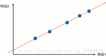
例如对于有2个特征的样本,现在对样本进行降维处理。首先考虑选择特征1或者特征2,经过降维后的样本如图所示。
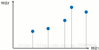
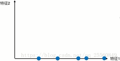

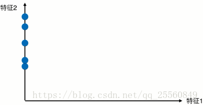
这个时候可以发现相对于选择特征2,选择特征1进行映射后,样本的可区分度更高。除了向某个特征做映射,还可以选择某个轴进行映射,例如下图所示的轴,样本经过映射后,可以有更大的间距。所以现在的问题就是如何找一个轴,使样本有最大的间距。
2.求解思路
事实上,可以使用方差来定义样本之间的间距。方差越大表示样本分布越稀疏,方差越小表示样本分布越密集。
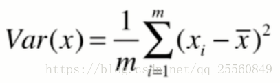
在求解方差前,可以先对样本减去每个特征的均值,这种处理方式不会改变样本的相对分布,并且求方差的公式可以转换成图示的公式。在这里,xi代表已经经过映射后的样本,此时xi每个维度上的均值都是0。
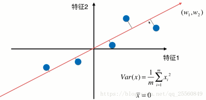
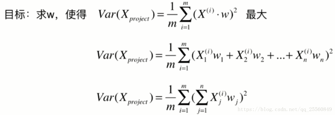
现在求一个轴的方向w=(w1,w2),使得映射到w之后方差最大。
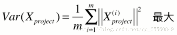

因此求解的公式可以转换成如下形式。
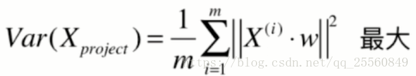
因此求解的目标转换成。这就转换成了求目标函数的最优化问题,可以通过梯度上升法进行求解。
二、梯度上升法求解
1.公式求解
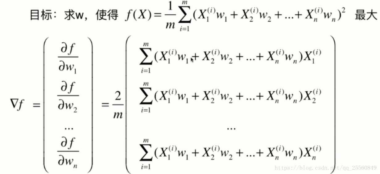
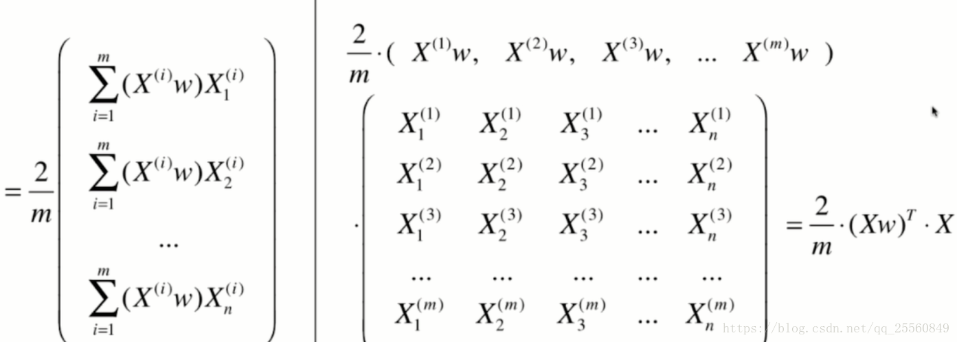
最终公式可以化简为如下形式。

2.代码实现
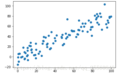
import numpy as np
import matplotlib.pyplot as plt
x = np.empty((100,2))
x[:,0]= np.random.uniform(0.,100.,size = 100)
x[:,1]= 0.75*x[:,0]+3.+np.random.normal(0,10.,size=100) #之所以让2个特征有一定的线性关系是为了使降维更明显
plt.scatter(x[:,0],x[:,1])
plt.show()
def demean(x):
    return x-np.mean(x,axis=0)  #对每个特征值进行求均值
def f (w,x):
    return np.sum((x.dot(w)**2))/len(x)
def df_math(w,x):
    return x.T.dot(x.dot(w))*2./len(x)
def direstion(w):
    return w /np.linalg.norm(w)  #将w进行归一化,因为w仅代表方向
def gradietn_ascent(df,x,initial_w,eta,n_iters = 1e4,epsilon=1e-8):
    w = direstion(initial_w)
    cur_iter =0
    while cur_iter <n_iters:
        gradient = df(w,x)
        last_w = w
        w = w+eta*gradient
        w = direstion(w)
        if(abs(f(w,x)-f(last_w,x))<epsilon):
            break
    return w
x_mean = demean(x)
initial_w = np.random.random(x.shape[1])#初始化不能为0向量
eta = 0.01
w=gradietn_ascent(df_math,x_mean,initial_w,eta)
plt.scatter(x_mean[:,0],x_mean[:,1])
plt.plot([0,w[0]*30],[0,w[1]*30],color = 'r')
plt.show()
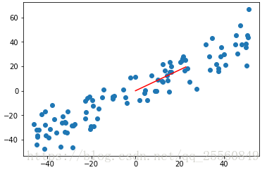
这里求得的仅仅是1个主成分,在更高维度的空间,可能还需要继续求出其他的主成分,即降更多的维度。
三、求前n个主成分
1.求解思路
在上面求解出了第一个主成分,即w=(w1,w2),为了求解第二个主成分,这里需要将数据在第一个主成分上的分量去除掉,这里使用的方法即空间几何的向量减法,得到的结果即下图中的绿线部分。
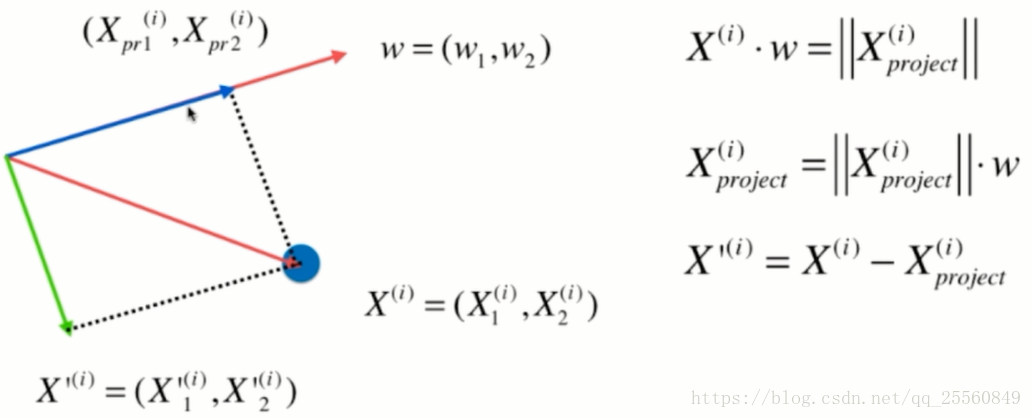
在得到绿线部分的分量后,再对该分量重新求第一主成分,以此类推,可以得到前n个主成分。
2.代码实现
def demean(x):
    return x-np.mean(x,axis=0)#对每个特征值进行求均值
def f (w,x):
    return np.sum((x.dot(w)**2))/len(x)
def df(w,x):
    return x.T.dot(x.dot(w))*2./len(x)

def demean(x):
    return x-np.mean(x,axis=0)#对每个特征值进行求均值
def f (w,x):
    return np.sum((x.dot(w)**2))/len(x)
def df(w,x):
    return x.T.dot(x.dot(w))*2./len(x)
def direstion(w):
    return w /np.linalg.norm(w)  #将w进行归一化,因为w仅代表方向
def first_conponent(df,x,initial_w,eta,n_iters = 1e4,epsilon=1e-8):
    w = direstion(initial_w)
    cur_iter =0
    while cur_iter <n_iters:
        gradient = df(w,x)
        last_w = w
        w = w+eta*gradient
        w = direstion(w)
        if(abs(f(w,x)-f(last_w,x))<epsilon):
            break
    return w
x_mean = demean(x)
initial_w = np.random.random(x.shape[1]) #初始化不能为0向量
eta = 0.01
w = first_conponent(df,x_mean,initial_w,eta)
x2 = np.empty(x.shape)
for i in range(len(x)):
x2[i] =x[i]-x[i].dot(w)*w
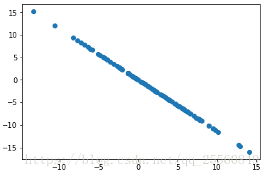
plt.scatter(x2[:,0],x2[:,1])
plt.show()
w2 = first_conponet(df,x2,initial_w,eta)
w2.dot(w)  #验证,结果接近0,第一主成分和第二主成分垂直,所以矩阵相乘为0
3.封装代码
def demean(x):
    return x-np.mean(x,axis=0)#对每个特征值进行求均值
def f (w,x):
    return np.sum((x.dot(w)**2))/len(x)
def df(w,x):
    return x.T.dot(x.dot(w))*2./len(x)
def direstion(w):
    return w /np.linalg.norm(w)  #将w进行归一化,因为w仅代表方向
def first_conponent(x,initial_w,eta,n_iters = 1e4,epsilon=1e-8):
    w = direstion(initial_w)
    cur_iter =0
    while cur_iter <n_iters:
        gradient = df(w,x)
        last_w = w
        w = w+eta*gradient
        w = direstion(w)
        if(abs(f(w,x)-f(last_w,x))<epsilon):
            break
    return w
def first_n_componets(n,x,eta=0.01,n_iters =1e4,epsilon=1e-8):
    x_pca = x.copy()
    x_pca = demean(x_pca)
    res =[]
    for i in range(n):
        initial_w = np.random.random(x_pca.shape[1])
        w = first_conponent(x_pca,initial_w,eta)
        res.append(w)

        x_pca = x_pca-x_pca.dot(w).reshape(-1,1)*w
    return res
first_n_componets(2,x)

上面仅仅使用2个特征值的样本,接下来使用真实的数据进行降维,并求原始样本向n个主成分降维的结果。
四、高维数据向底维数据转化
1.求解思路
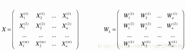
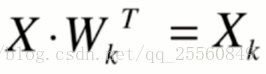
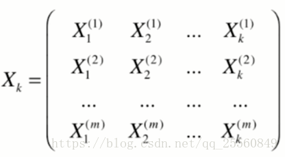
现在有原始样本x,并求得了前k个主成分,形成wk矩阵。现在需要将x映射到新的轴上,形成只有k个特征的新样本xk,用该样本来描述原来的样本x。
需要注意的是,这个时候数据已经丢失了一些信息,所以做逆运算时,并不能回到最初x的数据。
2.代码实现
import numpy as np

class PCA:

    def __init__(self, n_components):
        """初始化PCA"""
        assert n_components >= 1, "n_components must be valid"
        self.n_components = n_components
        self.components_ = None

    def fit(self, X, eta=0.01, n_iters=1e4):
        """获得数据集X的前n个主成分"""
        assert self.n_components <= X.shape[1], \
            "n_components must not be greater than the feature number of X"

        def demean(X):
            return X - np.mean(X, axis=0)

        def f(w, X):
            return np.sum((X.dot(w) ** 2)) / len(X)

        def df(w, X):
            return X.T.dot(X.dot(w)) * 2. / len(X)

        def direction(w):
            return w / np.linalg.norm(w)

        def first_component(X, initial_w, eta=0.01, n_iters=1e4, epsilon=1e-8):

            w = direction(initial_w)
            cur_iter = 0

            while cur_iter < n_iters:
                gradient = df(w, X)
                last_w = w
                w = w + eta * gradient
                w = direction(w)
                if (abs(f(w, X) - f(last_w, X)) < epsilon):
                    break

                cur_iter += 1

            return w

        X_pca = demean(X)
        self.components_ = np.empty(shape=(self.n_components, X.shape[1]))
        for i in range(self.n_components):
            initial_w = np.random.random(X_pca.shape[1])
            w = first_component(X_pca, initial_w, eta, n_iters)
            self.components_[i,:] = w

            X_pca = X_pca - X_pca.dot(w).reshape(-1, 1) * w

        return self

    def transform(self, X):
        """将给定的X,映射到各个主成分分量中"""
        assert X.shape[1] == self.components_.shape[1]

        return X.dot(self.components_.T)

    def inverse_transform(self, X):
        """将给定的X,反向映射回原来的特征空间"""
        assert X.shape[1] == self.components_.shape[0]

        return X.dot(self.components_)

    def __repr__(self):
        return "PCA(n_components=%d)" % self.n_components
使用代码:
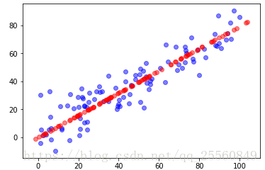
import numpy as np
import matplotlib.pyplot as plt
x = np.empty((100,2))
x[:,0]= np.random.uniform(0.,100.,size = 100)
x[:,1]= 0.75*x[:,0]+3.+np.random.normal(0,10.,size=100) #之所以让2个特征有一定的线性关系是为了使降维更明显
from ml.PCA import PCA
pca = PCA(n_components=1)
pca.fit(x)
x_reduction = pca.transform(x)
x_restore = pca.inverse_transform(x_reduction)
plt.scatter(x[:,0],x[:,1],color='b',alpha=0.5)
plt.scatter(x_restore[:,0],x_restore[:,1],color='r',alpha=0.5)
plt.show() #可以发现重新映射回原来矩阵形式时,只剩下主成分方向上的数据,restore的功能只是在高维的空间表达低维的样本
3.sklearn中的PCA
from sklearn.decomposition import PCA
pca = PCA(n_components=1)
pca.fit(x)
pca.components_

可以发现方向相反,接下来的降维和使用和上面自己编写的代码一样。需要注意的是,这里使用的降维方法并不是梯度上升法。
4.对手写识别数据进行降维
import numpy as np
import matplotlib.pyplot as plt
from sklearn import datasets
digits = datasets.load_digits()
x = digits.data
y = digits.target
from sklearn.model_selection import train_test_split
x_train,x_test,y_train,y_test = train_test_split(x,y,random_state = 666)
from sklearn.neighbors import KNeighborsClassifier
knn = KNeighborsClassifier()
knn.fit(x_train,y_train)
knn.score(x_test,y_test)
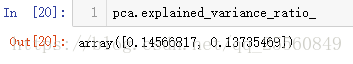
from sklearn.decomposition import PCA
pca = PCA(n_components=2)
pca.fit(x_train)
x_train_reduction = pca.transform(x_train)
x_test_reduction = pca.transform(x_test)#测试数据集也必须降维
knn = KNeighborsClassifier()
knn.fit(x_train_reduction,y_train)
knn.score(x_test_reduction,y_test)

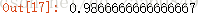
可以发现,经过降维后,因为维度就剩下2个,得出的分值很低,所以应该保留更多的特征值,但是具体保留多少特征合适?衡量的指标是什么?pca中有个变量为pca.explained_variance_ratio_,可以用来衡量得出来的新的映射空间保留了原始数据的多少方差。对于上面求得的结果,有如下。这代表经过映射后的数据,只保留原始数据大约百分之(14+13=27)的方差,丢掉了原来约73的方差,这个损失是比较大的。
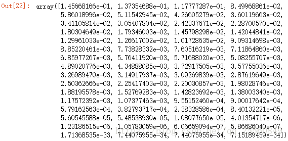
所以现在的问题是,我们应该保留多少的维度使得信息丢失在允许法范围内。假设我们选取的主成分的个数和原来的样本特征个数一样,这时候再观察explained_variance_ratio_发现,由于explained_variance_ratio_是按照大小顺序排列,越到后面,值越小,几乎可以忽略。
pca = PCA(n_components=x_train.shape[1]) #保留所有的维度
pca.fit(x_train)
pca.explained_variance_ratio_
现在将这些值进行累加并在坐标轴上展现出来。
plt.plot([i for i in range(x_train.shape[1])],[np.sum(pca.explained_variance_ratio_[:i+1]) for i in range(x_train.shape[1])])
plt.show()
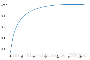
观察该图可以发现,当横轴为0时,纵轴也为0(丢失了所有信息),当横轴为特征值大小时,纵轴为1(保留了全部信息)。因此,比如想要保留95%的信息,就可以通过该图知道应该保留多少个特征信息。
pca = PCA(0.95) #传入的参数为0.95,代表保留的百分之多少的信息
pca.fit(x_train)
pca.n_components_  #结果为28
x_train_reduction = pca.transform(x_train)
x_test_reduction = pca .transform(x_test)
knn = KNeighborsClassifier()
knn.fit(x_train_reduction,y_train)
knn.score(x_test_reduction,y_test)
这个时候,发现分值明显得到了提高。而且如果进行时间测试,时间缩短了很多。
将数据降到2维,可以将高维度难以想象的数据,通过低维度进行展示,这里我们将手写识别数据进行展示。
pca = PCA(n_components=2)
pca.fit(x)
x_reduction = pca.transform(x)
for i in range(10):
    plt.scatter(x_reduction[y==i,0],x_reduction[y==i,1],alpha=0.8)
plt.show() #可以发现即使是2维,也有较好的区分度

5.MNIST数据集进行降维
import numpy as np
from sklearn.datasets import fetch_mldata
mnist = fetch_mldata("MNIST original") #第一次加载会需要一些时间
x,y = mnist['data'],mnist['target']
x_train = np.array(x[:60000],dtype=float)
y_train = np.array(y[:60000],dtype=float)
x_test = np.array(x[:60000],dtype=float)
y_test = np.array(y[60000:],dtype=float)
不实用pca时,直接经过knn会需要很长的时间。
from sklearn.neighbors import KNeighborsClassifier
knn = KNeighborsClassifier()
%time knn.fit(x_train,y_train)
%time knn.score(x_test,y_test)
使用pca后发现,时间提高很多,而且防止还提高了,这涉及到了pca的一个重要的作用-降噪。即在降维的过程中也将噪声减小了。
from sklearn.decomposition import PCA
pca = PCA(0.9)
pca.fit(x_train)
x_train_reduction = pca.transform(x_train)
x_test_reduction = pca.transform(x_test)#测试数据集也必须降维
knme knn.fit(x_train_reduction,y_train)
%time knn.score(x_test_reduction,y_test)
6.降噪
首先看之前的一个数据。
import numpy as np
import matplotlib.pyplot as plt
x = np.empty((100,2))
x[:,0]= np.random.uniform(0.,100.,size = 100)
x[:,1]= 0.75*x[:,0]+3.+np.random.normal(0,5.,size=100) #之所以让2个特征有一定的线性关系是为了使降维更明显
plt.scatter(x[:,0],x[:,1])
plt.show()
from sklearn.decomposition import PCA
pca = PCA(n_components=1)
pca.fit(x)
x_reduction = pca.transform(x)
x_restore = pca.inverse_transform(x_reduction)
plt.scatter(x[:,0],x[:,1],color='r')
plt.scatter(x_restore[:,0],x_restore[:,1])
plt.show()

原来的数据可能是因为测量的过程中出现了问题,所以发生了一定的抖动(即产生了噪声),经过降维后可以发现最终的数据在一条直线上,因此所pca有一定的降噪能力。下面使用手写识别例子继续探讨降维中的去燥功能。
from sklearn import datasets
digits = datasets.load_digits()
x = digits.data
y = digits.target
noisy_digits = x + np.random.normal(0,4,size=x.shape) #这里加入随机噪声
example_digits = noisy_digits[y==0,:][:10]
for num in range(1,10):
x_num = noisy_digits[y==num,:][:10]
example_digits = np.vstack([example_digits,x_num])#将全部样本按照0-10叠起来,共100个样本
def plot_digits(data): #这个函数当做模块使用即可,不必深究
fig,axes = plt.subplots(10,10,figsize=(10,10),subplot_kw={'xticks':[],'yticks':[]},gridspec_kw=dict(hspace=0.1,wspace=0.1))
for i,ax in enumerate(axes.flat):
ax.imshow(data[i].reshape(8,8),cmap='binary',interpolation='nearest',clim=(0,16))
plt.show()
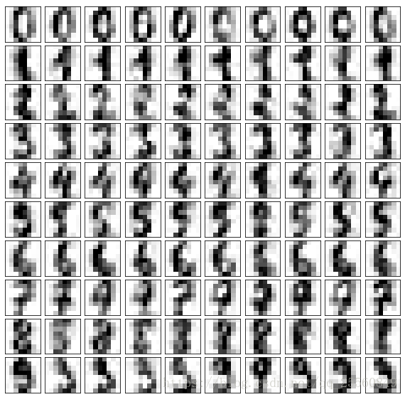
plot_digits(example_digits) #调用函数
可以看到图像十分模糊,现在通过pca进行降噪处理。

pca = PCA(0.5)
pca.fit(noisy_digits)
pca.n_components_components = pca.transform(example_digits)
filtered_digits = pca.inverse_transform(components)
plot_digits(filtered_digits)