1. 引言
上一篇日志中,我们最终推导出了计算最优系数的公式。
Logistic 回归数学公式推导
本文,我们就利用上一篇文章中计算出的公式来实现模型的训练和数据的分类。
2. 通过 python 实现 logistic 算法
有了上一篇日志中的公式,《机器学习实战》中的代码就非常容易理解了:
# -*- coding:UTF-8 -*-
# {{{
import matplotlib.pyplot as plt
import numpy as np


def loadDataSet():
    """
    生成数据矩阵与标签矩阵

    :return: 数据矩阵与标签矩阵
    """
    dataMat = []
    labelMat = []
    fr = open('test_dataset.txt')
    for line in fr.readlines():
        lineArr = line.strip().split()
        """ 每行数据钱添加特征 x0 """
        dataMat.append([1.0, float(lineArr[0]), float(lineArr[1])])
        labelMat.append(int(lineArr[2]))
    fr.close()
    return dataMat, labelMat


def sigmoid(inX):
    return 1.0 / (1 + np.exp(-inX))


def gradAscent(dataMatIn, classLabels):
    """
    梯度上升算法

    :param dataMatIn: 数据矩阵
    :param classLabels: 标签矩阵
    :return: 最有参数数组
    """
    dataMatrix = np.mat(dataMatIn)
    """ 转置 """
    labelMat = np.mat(classLabels).transpose()

    """ 获取矩阵行数 m 和列数 n """
    m, n = np.shape(dataMatrix)
    """ 迭代步长 """
    alpha = 0.001
    """ 迭代次数 """
    maxCycles = 500
    weights = np.ones((n, 1))
    for k in range(maxCycles):
        """ 带入数学公式求解 """
        h = sigmoid(dataMatrix * weights)
        weights = weights + alpha * dataMatrix.transpose() * (labelMat - h)
    """ 转换为 array """
    return weights.getA()


def plotBestFit(weights):
    """
    绘制数据集与结果分类线

    :param weights: 权重参数数组
    :return:
    """
    dataMat, labelMat = loadDataSet()
    dataArr = np.array(dataMat)

    """ 数据个数 """
    n = np.shape(dataMat)[0]

    """ 测试数据两组分类结果集 """
    xcord1 = []
    ycord1 = []
    xcord2 = []
    ycord2 = []

    """ 对数据进行分类 """
    for i in range(n):
        if int(labelMat[i]) == 1:
            xcord1.append(dataArr[i, 1])
            ycord1.append(dataArr[i, 2])
        else:
            xcord2.append(dataArr[i, 1])
            ycord2.append(dataArr[i, 2])

    """ 绘图 """
    fig = plt.figure()
    """ 分割画布为一整份,占据其中一整份 """
    ax = fig.add_subplot(111)
    """ 离散绘制分类结果为 1 的样本 """
    ax.scatter(xcord1, ycord1, s=20, c='red', marker='s', alpha=.5)
    """ 离散绘制分类结果为 0 的样本 """
    ax.scatter(xcord2, ycord2, s=20, c='green', alpha=.5)
    x1 = np.arange(-3.0, 3.0, 0.1)
    x2 = (-weights[0] - weights[1] * x1) / weights[2]
    ax.plot(x1, x2)
    plt.title('BestFit')
    plt.xlabel('X1')
    plt.ylabel('X2')
    plt.show()


if __name__ == '__main__':
    dataMat, labelMat = loadDataSet()
    weights = gradAscent(dataMat, labelMat)
    plotBestFit(weights)
# }}}
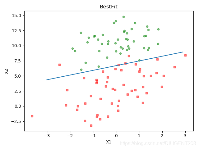
训练样本数据见本文的附录。
3. 随机梯度上升算法
当数据量达到上亿或更多数据以后,梯度上升算法中的矩阵乘法等操作显然耗时将上升到非常高的程度,那么,我们是否可以不用整个数据集作为样本来计算其权重参数而是只使用其中的一部分数据来训练呢?
这个算法思想就是随机梯度上升算法,他通过随机取数据集中的部分数据,来代表整体数据集,从而实现对数据样本集的缩小,达到减少计算量,降低算法时间复杂度的目的。
3.1. 算法代码
def randGradientAscent(dataMatrix, classLabels, numIter=20):
    """
    随机梯度上升算法

    :param dataMatrix: 数据矩阵
    :param classLabels: 标签矩阵
    :param numIter: 外循环次数
    :return: 权重数组与回归系数矩阵
    """
    time0 = time.time()
    m,n = np.shape(dataMatrix)
    weights = np.ones(n)
    weights_array = np.array([])
    innerIterNum = int(m/100)
    for j in range(numIter):
        dataIndex = list(range(m))
        for i in range(innerIterNum):
            alpha = 4/(1.0 + j + i) + 0.01  # 降低alpha的大小,每次减小1/(j+i)
            """ 随机选取样本 """
            randIndex = int(random.uniform(0,len(dataIndex)))
            chose = dataIndex[randIndex]
            h = sigmoid(sum(dataMatrix[chose]*weights))
            error = classLabels[chose] - h
            weights = weights + alpha * error * dataMatrix[chose]
            weights_array = np.append(weights_array,weights,axis=0)
            del(dataIndex[randIndex])
    weights_array = weights_array.reshape(numIter*innerIterNum, n)
    print("随机梯度算法耗时:", time.time() - time0)
    return weights, weights_array
上述代码与梯度上升算法相比,主要有以下改进:
- 将原有的迭代 + 矩阵操作替换成内外层双层循环实现,内循环只随机选取原数据集的 1/100 规模,从而实现计算量的缩减
- alpha 动态调整,随着内循环的进行,逐步缩小,从而对获取更准确的最优值与运行时间二者的优化
4. 随机梯度上升算法与梯度上升算法效果对比
下面代码对比了梯度上升算法与随机梯度上升算法的效果。
# -*- coding:UTF-8 -*-
# {{{
import time

from matplotlib.font_manager import FontProperties
import matplotlib.pyplot as plt
import numpy as np
import random


def loadDataSet():
    """
    加载数据

    :return: 数据集,标签集
    """
    dataMat = []
    labelMat = []
    fr = open('test_dataset.txt')
    for line in fr.readlines():
        for i in range(100):
            lineArr = line.strip().split()
            dataMat.append([1.0, float(lineArr[0]), float(lineArr[1])])
            labelMat.append(int(lineArr[2]))
    fr.close()
    return dataMat, labelMat


def sigmoid(inX):
    return 1.0 / (1 + np.exp(-inX))


def gradAscent(dataMatIn, classLabels, maxCycles = 300):
    """
    梯度上升算法

    :param dataMatIn: 数据矩阵
    :param classLabels: 数据集
    :param maxCycles: 迭代次数
    :return: 权重数组与回归系数矩阵
    """
    time0 = time.time()
    dataMatrix = np.mat(dataMatIn)
    labelMat = np.mat(classLabels).transpose()
    m, n = np.shape(dataMatrix)
    alpha = 0.0001
    weights = np.ones((n,1))
    weights_array = np.array([])
    for k in range(maxCycles):
        h = sigmoid(dataMatrix * weights)
        error = labelMat - h
        weights = weights + alpha * dataMatrix.transpose() * error
        weights_array = np.append(weights_array,weights)
    weights_array = weights_array.reshape(maxCycles,n)
    print("梯度上升算法耗时:", time.time() - time0)
    return weights.getA(), weights_array


def randGradientAscent(dataMatrix, classLabels, numIter=20):
    """
    随机梯度上升算法

    :param dataMatrix: 数据矩阵
    :param classLabels: 标签矩阵
    :param numIter: 外循环次数
    :return: 权重数组与回归系数矩阵
    """
    time0 = time.time()
    m,n = np.shape(dataMatrix)
    weights = np.ones(n)
    weights_array = np.array([])
    innerIterNum = int(m/100)
    for j in range(numIter):
        dataIndex = list(range(m))
        for i in range(innerIterNum):
            alpha = 4/(1.0 + j + i) + 0.01  #降低alpha的大小,每次减小1/(j+i)
            """ 随机选取样本 """
            randIndex = int(random.uniform(0,len(dataIndex)))
            chose = dataIndex[randIndex]
            h = sigmoid(sum(dataMatrix[chose]*weights))
            error = classLabels[chose] - h
            weights = weights + alpha * error * dataMatrix[chose]
            weights_array = np.append(weights_array,weights,axis=0)
            del(dataIndex[randIndex])
    weights_array = weights_array.reshape(numIter*innerIterNum, n)
    print("随机梯度算法耗时:", time.time() - time0)
    return weights, weights_array


def plotWeights(rand_gradientascent_weights, gradient_ascent_weights):
    """
    绘制回归系数与迭代次数的关系

    :param rand_gradientascent_weights: 随机梯度上升权重矩阵
    :param gradient_ascent_weights: 梯度上升权重矩阵
    :return:
    """

    font = FontProperties(fname=r"c:\windows\fonts\simsun.ttc", size=14)
    """
    将fig画布分隔成1行1列,不共享x轴和y轴,fig画布的大小为 (13,8),分为六个区域
    """
    fig, axs = plt.subplots(nrows=3, ncols=2, sharex='none', sharey='none', figsize=(20,10))

    x1 = np.arange(0, len(rand_gradientascent_weights), 1)
    axs[0][0].plot(x1, rand_gradientascent_weights[:, 0])
    axs0_title_text = axs[0][0].set_title(u'改进的随机梯度上升算法:回归系数与迭代次数关系',FontProperties=font)
    axs0_ylabel_text = axs[0][0].set_ylabel(u'W0',FontProperties=font)
    plt.setp(axs0_title_text, size=20, weight='bold', color='black')
    plt.setp(axs0_ylabel_text, size=20, weight='bold', color='black')

    axs[1][0].plot(x1, rand_gradientascent_weights[:, 1])
    axs1_ylabel_text = axs[1][0].set_ylabel(u'W1',FontProperties=font)
    plt.setp(axs1_ylabel_text, size=20, weight='bold', color='black')

    axs[2][0].plot(x1, rand_gradientascent_weights[:, 2])
    axs2_xlabel_text = axs[2][0].set_xlabel(u'迭代次数',FontProperties=font)
    axs2_ylabel_text = axs[2][0].set_ylabel(u'W1',FontProperties=font)
    plt.setp(axs2_xlabel_text, size=20, weight='bold', color='black')
    plt.setp(axs2_ylabel_text, size=20, weight='bold', color='black')


    x2 = np.arange(0, len(gradient_ascent_weights), 1)
    axs[0][1].plot(x2, gradient_ascent_weights[:, 0])
    axs0_title_text = axs[0][1].set_title(u'梯度上升算法:回归系数与迭代次数关系',FontProperties=font)
    axs0_ylabel_text = axs[0][1].set_ylabel(u'W0',FontProperties=font)
    plt.setp(axs0_title_text, size=20, weight='bold', color='black')
    plt.setp(axs0_ylabel_text, size=20, weight='bold', color='black')

    axs[1][1].plot(x2, gradient_ascent_weights[:, 1])
    axs1_ylabel_text = axs[1][1].set_ylabel(u'W1',FontProperties=font)
    plt.setp(axs1_ylabel_text, size=20, weight='bold', color='black')

    axs[2][1].plot(x2, gradient_ascent_weights[:, 2])
    axs2_xlabel_text = axs[2][1].set_xlabel(u'迭代次数',FontProperties=font)
    axs2_ylabel_text = axs[2][1].set_ylabel(u'W1',FontProperties=font)
    plt.setp(axs2_xlabel_text, size=20, weight='bold', color='black')
    plt.setp(axs2_ylabel_text, size=20, weight='bold', color='black')

    plt.show()


if __name__ == '__main__':
    dataMat, labelMat = loadDataSet()
    weights1,weights_array1 = randGradientAscent(np.array(dataMat), labelMat)
    weights2,weights_array2 = gradAscent(dataMat, labelMat)
    plotWeights(weights_array1, weights_array2)
# }}}
首先将数据集通过复制 100 次,从而实现将原有训练数据集从 100 个变为 10000 个的效果。
然后,我们画出了迭代过程中的权重变化曲线。
4.1. 输出结果
输出了:
随机梯度算法耗时: 0.03397965431213379
梯度上升算法耗时: 0.11360883712768555

4.2. 结果分析
可以看到,两个算法都刚好在我们迭代结束时趋于平衡,这是博主为了对比两个算法运行的时间对迭代次数进行多次调整的结果。
结果已经非常明显,虽然从波动范围来看,随机梯度上升算法在迭代过程中更加不稳定,但随机梯度上升算法的收敛时间仅仅是梯度上升算法的30%,时间大为缩短,如果数据规模进一步上升,则差距将会更加明显。
而从结果看,两个算法的最终收敛位置是非常接近的,但是,从原理上来说,随机梯度算法效果确实可能逊于梯度上升算法,但这仍然取决于步进系数、内外层循环次数以及随机样本选取数量的选择。
5. 《机器学习实战》随机梯度上升算法讲解中的错误
几天前,阅读《机器学习实战》时,对于作者所写的代码例子,有很多疑问,经过几天的研究,确认是某种原因导致的谬误,最终有了上文中博主自己改进过的代码,实现了文中的算法思想。
这里详细来说一下书中源码和结论中存在的纰漏。
下面代码是书中的源代码:
def stocGradAscent1(dataMatrix, classLabels, numIter=150):
    m,n = shape(dataMatrix)
    weights = ones(n)   #initialize to all ones
    for j in range(numIter):
        dataIndex = range(m)
        for i in range(m):
            alpha = 4/(1.0+j+i)+0.0001    #apha decreases with iteration, does not
            randIndex = int(random.uniform(0, len(dataIndex)))#go to 0 because of the constant
            h = sigmoid(sum(dataMatrix[randIndex]*weights))
            error = classLabels[randIndex] - h
            weights = weights + alpha * error * dataMatrix[randIndex]
            del(dataIndex[randIndex])
    return weights
这段代码存在下面的几个问题,尽信书不如无书,网上很多笔记和博客都是照搬书上的代码和结论,而没有进行自己的思考,这样是不可取的。
5.1. 随机样本选择时下标问题
代码中,randIndex 是从 0 到 dataIndex 长度 - 1的随机数,假设训练数据规模为 100。
那么首次迭代中,dataIndex 是从 0 到 99 的随机数,假设 dataIndex 取到的是 0,那么本次迭代的训练数据是第 0 条数据,然后,首次迭代的最后,删除了 dataIndex 的第 0 个元素。
第二次迭代中,dataIndex 是从 0 到 98 的随机数,假设 dataIndex 取到的是 0,那么本次迭代的训练数据是第 0 条数据,然后,第二次迭代的最后,删除了 dataIndex 的第 0 个元素。
。。。
如果刚好我们的 dataIndex 每次都取到 0,那么最终的训练结果将毫无意义。
首先,即使这段代码是正确的,del(dataIndex[randIndex]) 的意义是什么呢?dataIndex 列表存在的价值又是什么呢?为什么不直接用一个数字代表规模来进行每次内迭代中的自减操作呢?
所以代码原意是:
randIndex = dataIndex[int(random.uniform(0, len(dataIndex)))]
这样才是正确的。
5.2. 为什么内迭代 m 次
内迭代 m 次的结果是什么呢?是将数据集按行打乱顺序。
从矩阵运算的规则来看,将矩阵运算变成每一行拆分运算,其结果是完全等价的,而 python 算法库中,矩阵运算是通过 CPython 转化为 C 语言进行的,其运算速度是要明显优于我们自己拆分运算的。
对于整个算法来说,打乱样本数据的排列是完全没有任何意义的。
而事实上,在《机器学习实战》的文中,也提到,随机梯度上升算法是通过选取样本数据集的子集进行计算来实现效率的提升的,而这个思想并不是代码中所反映出的思想。
5.3. 随机梯度算法收敛速度更快
作者在运行结果中,对比了随机梯度上升算法与梯度上升算法达到收敛时的迭代次数。
首先,迭代内部算法不同,单纯比较迭代次数有什么意义呢?
而作者竟然将上述代码的外循环次数与梯度上升算法的迭代次数进行比较,这样的比较结果是在愚弄读者吧?
5.4. 随机选取机制可以减小波动?
书中对比随机梯度算法与梯度上升算法的权重迭代曲线,得出结论:这里的系数没有像之前那样出现周期性波动,这归功于样本随机选择机制。
无论是算法原理还是从作者贴出的图来看都不能得到这样的结论。
6. 附录
6.1. 训练样本数据
-0.017612       14.053064       0
-1.395634       4.662541        1
-0.752157       6.538620        0
-1.322371       7.152853        0
0.423363        11.054677       0
0.406704        7.067335        1
0.667394        12.741452       0
-2.460150       6.866805        1
0.569411        9.548755        0
-0.026632       10.427743       0
0.850433        6.920334        1
1.347183        13.175500       0
1.176813        3.167020        1
-1.781871       9.097953        0
-0.566606       5.749003        1
0.931635        1.589505        1
-0.024205       6.151823        1
-0.036453       2.690988        1
-0.196949       0.444165        1
1.014459        5.754399        1
1.985298        3.230619        1
-1.693453       -0.557540       1
-0.576525       11.778922       0
-0.346811       -1.678730       1
-2.124484       2.672471        1
1.217916        9.597015        0
-0.733928       9.098687        0
-3.642001       -1.618087       1
0.315985        3.523953        1
1.416614        9.619232        0
-0.386323       3.989286        1
0.556921        8.294984        1
1.224863        11.587360       0
-1.347803       -2.406051       1
1.196604        4.951851        1
0.275221        9.543647        0
0.470575        9.332488        0
-1.889567       9.542662        0
-1.527893       12.150579       0
-1.185247       11.309318       0
-0.445678       3.297303        1
1.042222        6.105155        1
-0.618787       10.320986       0
1.152083        0.548467        1
0.828534        2.676045        1
-1.237728       10.549033       0
-0.683565       -2.166125       1
0.229456        5.921938        1
-0.959885       11.555336       0
0.492911        10.993324       0
0.184992        8.721488        0
-0.355715       10.325976       0
-0.397822       8.058397        0
0.824839        13.730343       0
1.507278        5.027866        1
0.099671        6.835839        1
-0.344008       10.717485       0
1.785928        7.718645        1
-0.918801       11.560217       0
-0.364009       4.747300        1
-0.841722       4.119083        1
0.490426        1.960539        1
-0.007194       9.075792        0
0.356107        12.447863       0
0.342578        12.281162       0
-0.810823       -1.466018       1
2.530777        6.476801        1
1.296683        11.607559       0
0.475487        12.040035       0
-0.783277       11.009725       0
0.074798        11.023650       0
-1.337472       0.468339        1
-0.102781       13.763651       0
-0.147324       2.874846        1
0.518389        9.887035        0
1.015399        7.571882        0
-1.658086       -0.027255       1
1.319944        2.171228        1
2.056216        5.019981        1
-0.851633       4.375691        1
-1.510047       6.061992        0
-1.076637       -3.181888       1
1.821096        10.283990       0
3.010150        8.401766        1
-1.099458       1.688274        1
-0.834872       -1.733869       1
-0.846637       3.849075        1
1.400102        12.628781       0
1.752842        5.468166        1
0.078557        0.059736        1
0.089392        -0.715300       1
1.825662        12.693808       0
0.197445        9.744638        0
0.126117        0.922311        1
-0.679797       1.220530        1
0.677983        2.556666        1
0.761349        10.693862       0
-2.168791       0.143632        1
1.388610        9.341997        0
0.317029        14.739025       0
欢迎关注微信公众号

参考资料
Peter Harrington 《机器学习实战》。
李航 《统计学习方法》。
https://en.wikipedia.org/wiki/Maximum_likelihood_estimation。
https://en.wikipedia.org/wiki/Gradient_descent。
https://blog.csdn.net/c406495762/article/details/77851973。
https://blog.csdn.net/charlielincy/article/details/71082147。