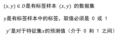
1 问题描述
MNIST 数据集来自美国国家标准与技术研究所, National Institute of Standards and Technology (NIST).数据集由来自 250 个不同人手写的数字构成, 其中 50% 是高中学生, 50% 来自人口 普查局 (the Census Bureau) 的工作人员
2 数据集获取
2.1 网站获取: http://yann.lecun.com/exdb/mnist/
2.2 TensorFlow提供了数据集读取方法
#导入TensorFlow
import tensorflow as tf
#导入读取方法
import tensorflow.examples.tutorials.mnist.input_data as input_data
#读入数据集
mnist = input_data.read_data_sets("MNIST_data/",one_hot = True)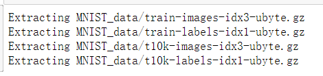
注:MNIST数据集文件在读取时如果指定目录下不存在,则会自动去下载,需等待一定时间如果已经存在了,则直接读取
3 了解数据集
print("训练集 train 数量:",mnist.train.num_examples,
      ",验证集 validation 数量:",mnist.validation.num_examples,
      ",测试集 test 数量:",mnist.test.num_examples
     )
print("train images shape:",mnist.train.images.shape,
     "lables shaple:",mnist.train.labels.shape)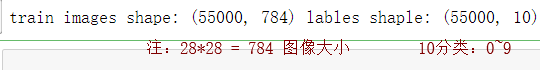
3.1 看具体image的数据
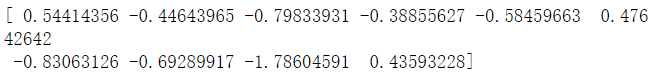
print(len(mnist.train.images[0]), mnist.train.images[0].shape)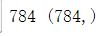 mnist.train.images[0]
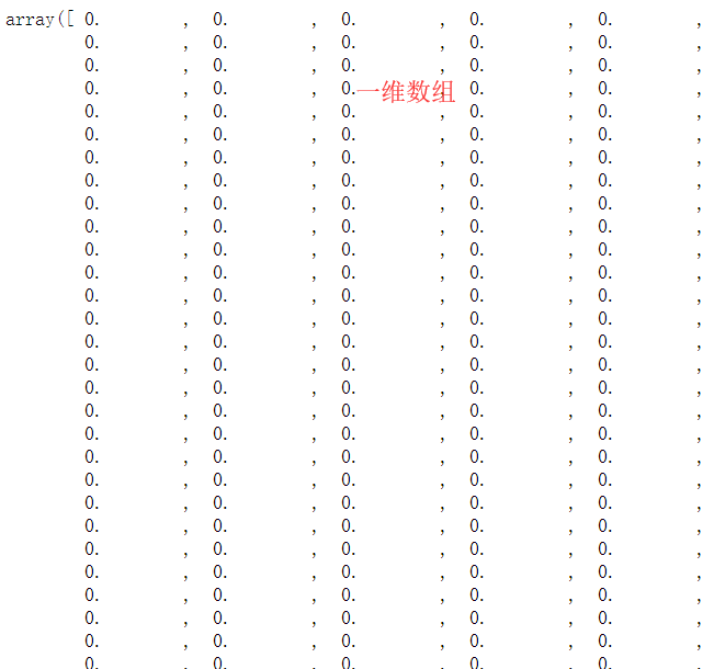 # image数据再塑性reshape mnist.train.images[0].reshape(28,28)
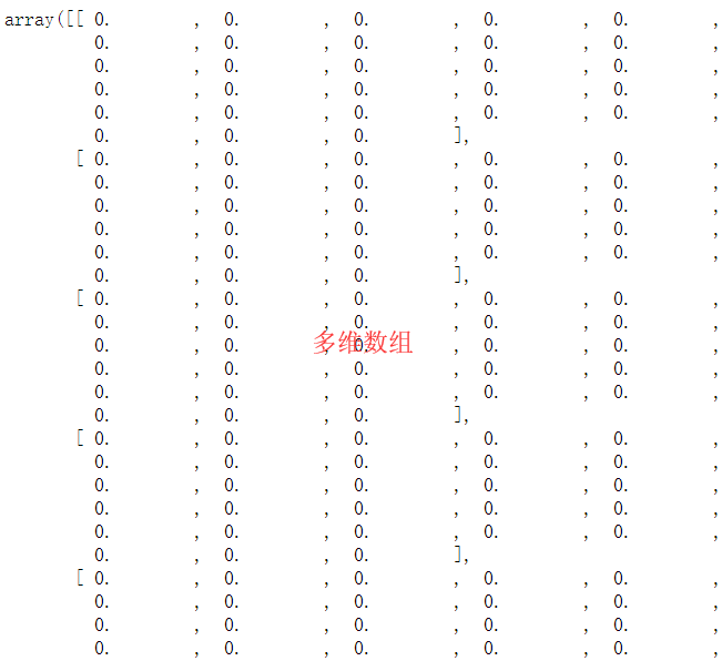
#可视化image
#定义函数
import matplotlib.pyplot as plt

def plot_image(image):
    plt.imshow(image.reshape(28,28),cmap = "binary")
    plt.show()
plot_image(mnist.train.images[3424])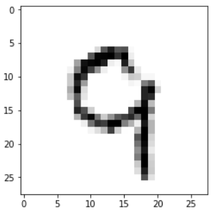
3.2 reshape() 函数
import numpy as np int_array = np.array([i for i in range(64)]) print(int_array)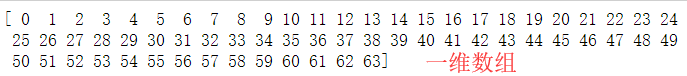 int_array.reshape(4,16)
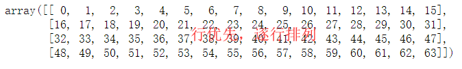 plt.imshow(mnist.train.images[454].reshape(14,56),cmap = "binary") plt.show()
3.3数据的批量读取
3.3.1 python切片
print(mnist.train.labels[0:10])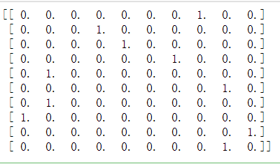
3.3.2 函数读取
# next_batch () 实现内部会对数据集先做shuffle处理
batch_images_xs,batch_labels_ys = mnist.train.next_batch(batch_size=10)
print(batch_labels_ys)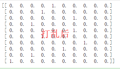
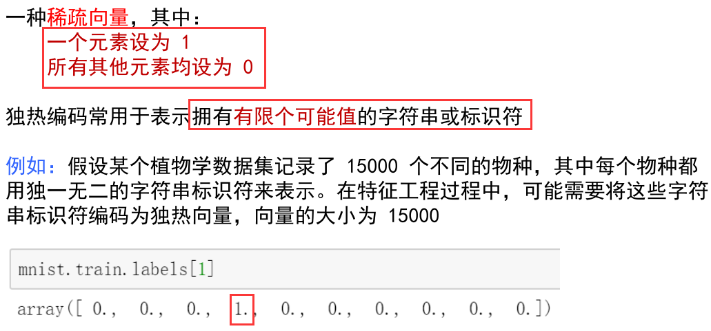
4 标签数据和独热编码
4.1标签数据
#打印image
plot_image(mnist.train.images[1])
# 打印imag对应的标签
print(mnist.train.labels[1])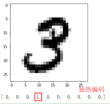
4.2 独热编码
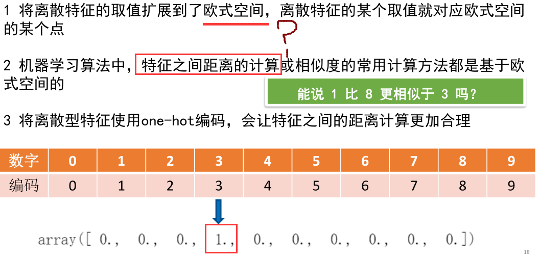
4.2.1 为什么要采用 one hot 编码
4.2.2如何从独热编码取值?
import numpy as np
# 打印imag对应的标签
print(mnist.train.labels[1])
# argmax 返回的是最大数的索引
np.argmax(mnist.train.labels[1])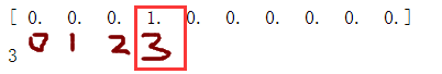
4.3 非one-hot编码的标签值
mnist_no_one_hot = input_data.read_data_sets("MNIST_data/",one_hot=False)
print(mnist_no_one_hot.train.labels[0:10])
5 数据集的划分
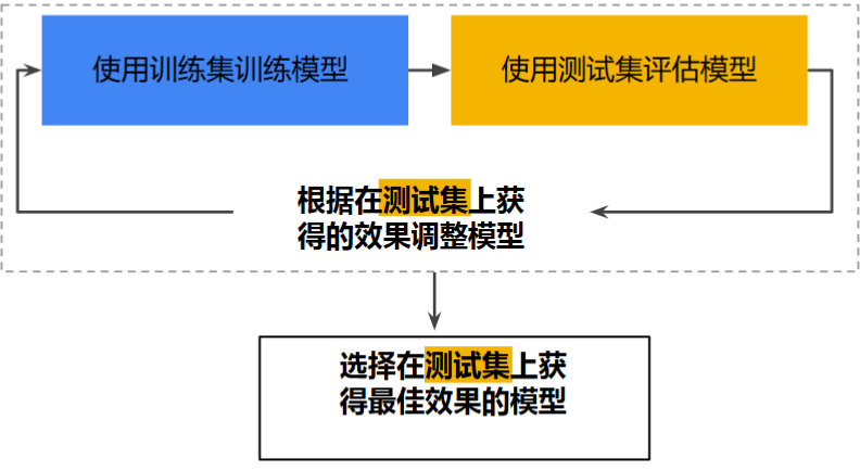
5.1 第一种划分
训练集 - 用于训练模型的子集集
测试集 - 用于测试模型的子集
确保测试集满足以下两个条件:
规模足够大,可产生具有统计意义的结果
能代表整个数据集,测试集的特征应该与训练集的特征相同5.1.1工作流程
5.1.2 存在的问题
多次重复执行该流程可能导致模型不知不觉地拟合了特定测试集的特性
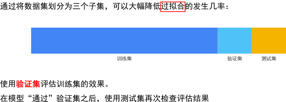
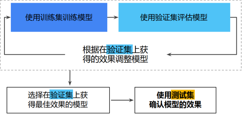
5.2 第二种划分
训练集 - 用于训练模型的子集集
验证集 - 用于验证模型的子集
测试集 - 用于测试模型的子集
5.2.1工作流程
5.3 数据验证
#读取验证数据
print("验证图像:",mnist.validation.images.shape,
     "标签:",mnist.validation.labels.shape)
#读取测试数据
print("测试图像:",mnist.test.images.shape,
     "标签:",mnist.test.labels.shape)
#读取训练数据
print("训练图像:",mnist.train.images.shape,
     "标签:",mnist.train.labels.shape)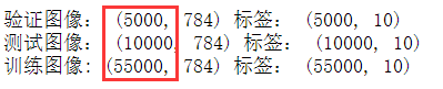
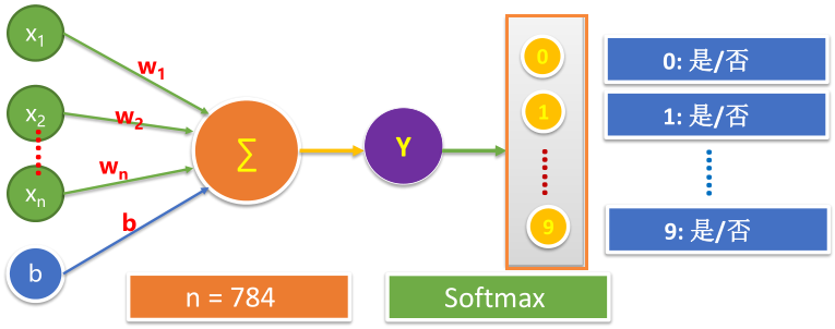
6 模型构建
6.1 定义待输入数据的占位符
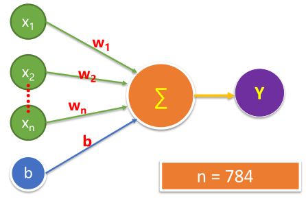
#mnist 中每张图片共有28*28 = 784个像素点
x = tf.placeholder(tf.float32,[None,784],name="X")
y = tf.placeholder(tf.float32,[None,10],name="Y")
6.2 定义模型变量
以正态分布的随机数初始化权重W,以常数0初始化偏置b
#定义变量
W = tf.Variable(tf.random_normal([784,10],name="W"))
b = tf.Variable(tf.zeros([10]),name="b")
6.3 了解 tf.random_normal ()
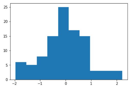
#生成100个随机数
norm = tf.random_normal([100])
with tf.Session() as sess:
    norm_data = norm.eval()
#打印前10个随机数
print(norm_data[:10])
#图形化打印出来
import matplotlib.pyplot as plt
plt.hist(norm_data)
plt.show()
6.4 定义前向计算
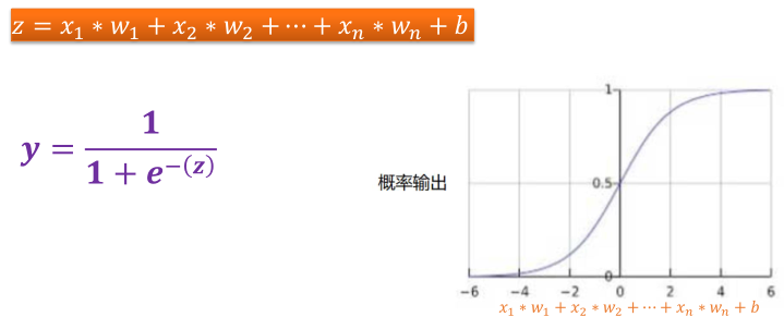
# matmul叉乘,前向计算
forward = tf.matmul(x,W) + b
6.4.1 结果分类
# Softmax 分类
pred = tf.nn.softmax(forward)
7 逻辑回归
许多问题的预测结果是一个在连续空间的数值,比如房价预测问题,可以用线性模型来描述:
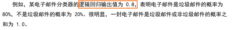
但也有很多场景需要输出的是概率估算值,例如:
• 根据邮件内容判断是垃圾邮件的可能性
• 根据医学影像判断肿瘤是恶性的可能性
• 手写数字分别是 0、1、2、3、4、5、6、7、8、9的可能性(概率)
这时需要将预测输出值控制在 [0,1]区间内
二元分类问题的目标是正确预测两个可能的标签中的一个【结果只有一个】
逻辑回归(Logistic Regression)可以用于处理这类问题7.1 Sigmod 函数
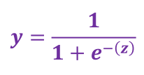
逻辑回归模型如何确保输出值始终落在 0 和 1 之间。
Sigmod函数(S型函数)生成的输出值正好具有这些特性,其定义如下:
定义域为全体实数,值域在[0,1]之间
Z值在0点对应的结果为0.5
sigmoid函数连续可微分7.1.1 特定样本的逻辑回归模型的输出
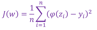
7.2 逻辑回归中的损失函数
线性回归的损失函数是平方损失,如果逻辑回归的损失函数也为平方损失,则:
其中:
将Sigmoid函数带入上述函数
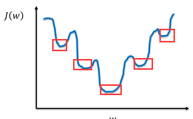
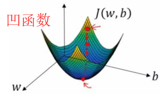
非凸函数,有多个极小值
如果采用梯度下降法,会容易导致陷入局部最优解中
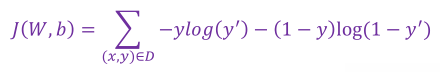
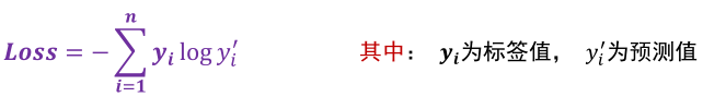
7.2.1 二元逻辑回归的损失函数采用 “对数损失函数” :
其中:
8 多元分类
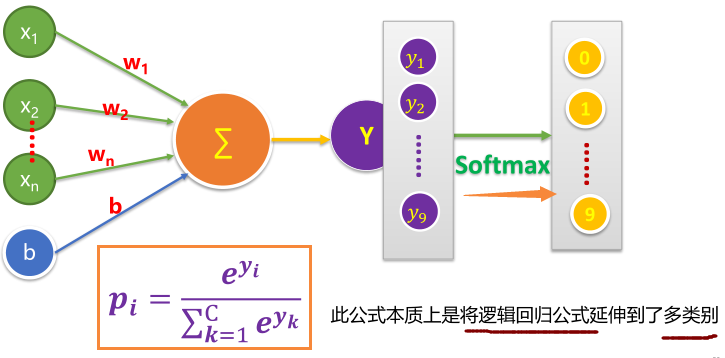
8.1 Softmax 思想
逻辑回归可生成介于0-1.0之间的小数
Softmax将这一想法延伸到多类别领域
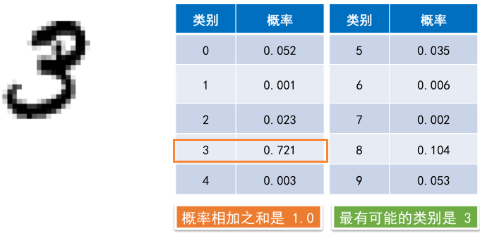
在多累别问题中,Softmax会为每一个分类分配一个用小数表示的概率,这些小数表示的概率相加之和为1.0
8.2 Softmax实例
8.3神经网络中的Softmax层
8.4 Softmax方程式
8.5 Softmax举例
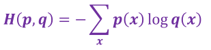
8.6 交叉熵损失函数
交叉熵是信息论中的概念,原为估算平均编码长度的。给定两个概率分布p和q,通过q来表示p的交叉熵
交叉熵表示的是两个概率分布之间的距离,p表示正确答案,q表示预测值,交叉熵越小,两个概率分布越接近
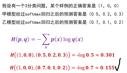
8.7 交叉熵损失函数计算实例
8.8 定义交叉熵损失函数
# 定义损失函数
loss_function = tf.reduce_mean( -tf.reduce_sum (y * tf.log(pred),reduction_indices = 1))
8.9 argmax()用法
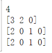
#载入数据
import tensorflow as tf
import numpy as np

arr1 = np.array([1,3,2,5,7,0])
arr2 = np.array([[1.0,2,3],[3,2,1],[4,7,2],[8,3,2]])
print(arr1)
print(arr2)
argmax_1 = tf.argmax(arr1)
argmax_20 = tf.argmax(arr2,0) #指定参数为0,按第一维(行)的元素取值,即同列的每一行
argmax_21 = tf.argmax(arr2,1) #指定参数为1,按第二维(列)的元素取值,即同行的每一列
argmax_22 = tf.argmax(arr2,-1)#指定参数为-1,即第最后维的元素取值

with tf.Session() as sess:
    print(argmax_1.eval())
    print(argmax_20.eval())
    print(argmax_21.eval())
    print(argmax_22.eval())
9 分类模型构建与训练实践
9.1载入数据
#载入数据
import tensorflow as tf
from tensorflow.examples.tutorials.mnist import input_data
mnist = input_data.read_data_sets("MNIST_data/",one_hot = True)
9.2 定义占位符
# mnist 中每张图片共有28*28=784个像素点
x = tf.placeholder(tf.float32,[None,784],name="X")
# 0 -9 一共10个数字 ,10个类别
y = tf.placeholder(tf.float32,[None,10],name = "Y")
9.3变量定义
#定义变量
W = tf.Variable(tf.random_normal([784,10],name = "W"))
b = tf.Variable(tf.zeros([10]),name="b")
神经网络中,权值W的初始值设为正态分布的随机数,偏置项b的初始值为1 -10的随机数或常数。
9.4单个神经元构建神经网络
#向前计算
forward = tf.matmul(x,W) + b
9.5 softmax 分类
#softmax分类
pred = tf.nn.softmax(forward)
Softmax Regression 会对每一类别估计出一个概率
工作原理:判定为某一类的特征相加,然后将这些特征转化为判定是这类的概率9.6 设置训练参数
train_epochs = 50   #训练轮数
batch_size = 100  #单次训练样本数【批次大小】
total_batch = int(mnist.train.num_examples/batch_size)  #一轮训练有多少批次
display_step = 1  #显示粒度
learning_rate = 0.01 #学习率
9.7 定义损失函数
# 定义损失函数
loss_function = tf.reduce_mean( -tf.reduce_sum (y * tf.log(pred),reduction_indices = 1))
9.8 选择优化器
# 选择优化器【梯度下降】
optimizer = tf.train.GradientDescentOptimizer(learning_rate).minimize(loss_function)
9.9 定义准确率
#检查预测类别tf.argmax(pred,1)与实际类别tf.argmax(y,1)的匹配情况
correct_prediction = tf.equal(tf.argmax(pred,1),tf.argmax(y,1))
# 准确率,将布尔值转化为浮点数,计算平均值
accuracy = tf.reduce_mean(tf.cast(correct_prediction,tf.float32))
9.10 会话声明
#声明会话
sess = tf.Session()
#变量初始化
init = tf.global_variables_initializer()
sess.run(init)
9.11 模型训练
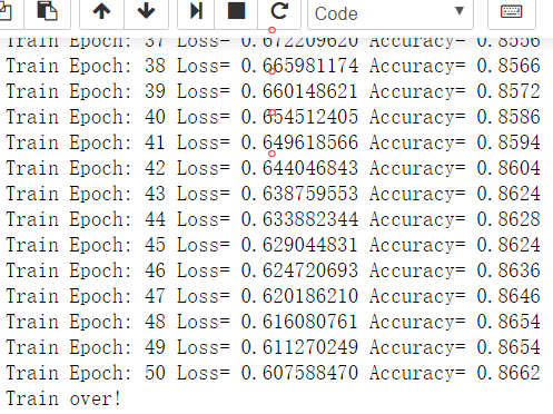
#开始训练
for epoch in range(train_epochs):
    for batch in range(total_batch):
        xs,ys = mnist.train.next_batch(batch_size) #读取批次数据
        sess.run(optimizer,feed_dict={x:xs,y:ys})  #执行批次训练

    #total_batch 个批次训练后,使用验证数据计算误差与准确性,验证集没有分批
    loss,acc = sess.run([loss_function,accuracy],
        feed_dict = {x: mnist.validation.images ,y: mnist.validation.labels})

    #打印训练过程中的详细信息
    if(epoch+1) % display_step == 0:
        print("Train Epoch:",'%02d' % (epoch+1),"Loss=", "{:.9f}".format(loss),"Accuracy=","{:.4f}".format(acc))

print("Train over!")
结果:损失值Loss是趋于更小的,准确率Accuracy 越来 越高
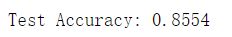
9.12 测试模型
在测试集中评估准确率
accu_test = sess.run(accuracy,feed_dict = {x:mnist.test.images,y:mnist.test.labels})
print("Test Accuracy:",accu_test)
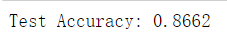
在验证集中评估准确率
accu_validation = sess.run(accuracy,feed_dict = {x:mnist.validation.images,y:mnist.validation.labels})
print("Test Accuracy:",accu_validation)
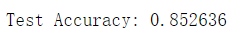
在训练集中评估准确率
accu_train = sess.run(accuracy,feed_dict = {x:mnist.train.images,y:mnist.train.labels})
print("Test Accuracy:",accu_train)
10 模型训练和可视化
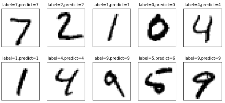
10.1 进行预测
在建立模型并进行训练后,若认为准确率可以接受,则使用此模型进行预测
# 由于pred 预测结果是one_hot 编码格式,所以需要转换成0 — 9数字
prediction_result = sess.run(tf.argmax(pred,1),feed_dict={x:mnist.test.images})
10.2 查看预测结果
#查看预测结果中的前10项
prediction_result[0:15]
10.3 定义可视化函数
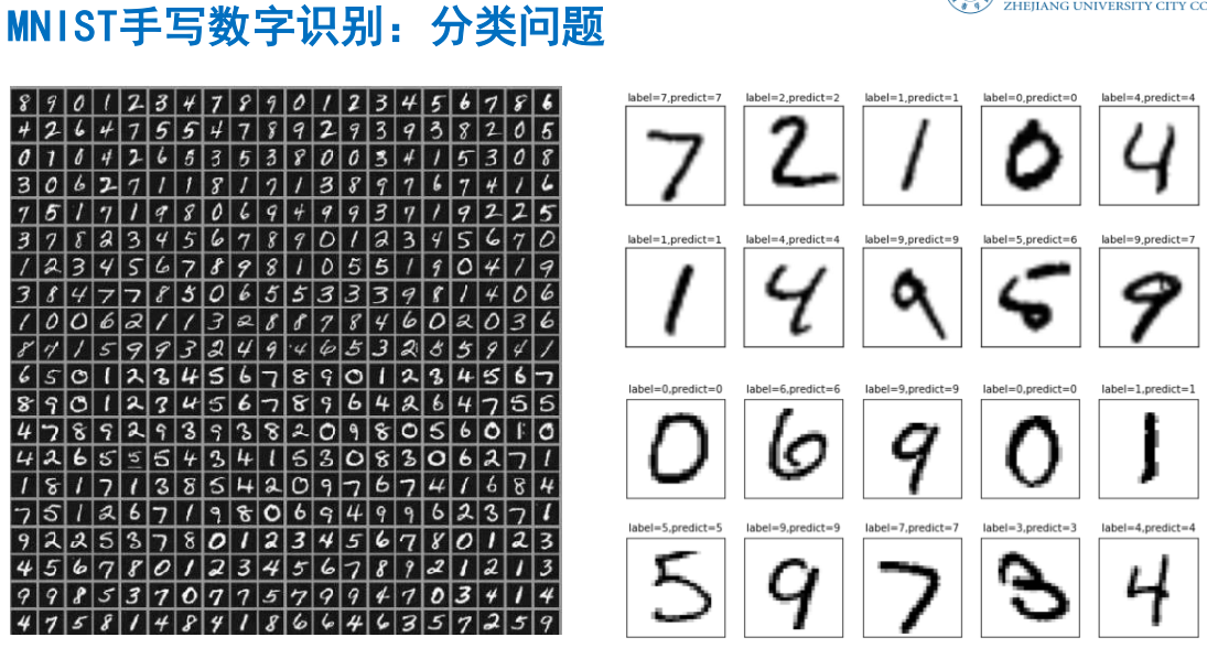
#定义可视化函数
import matplotlib.pyplot as plt
import numpy as np
def plot_images_labels_prediction(images, #图像列表
                                  labels, #标签列表
                                  prediction, #预测值列表
                                  index, #从第index个开始显示
                                  num = 10 ): #缺省一次显示10幅
    fig = plt.gcf() #获取当前图表,
    fig.set_size_inches(10,12) # 一英寸为2.54cm
    if num > 25:
        num = 25   #最多显示25个子图
    for i in range (0,num):
        ax = plt.subplot(5,5,i+1)  #获取当前要处理的子图

        ax.imshow(np.reshape(images[index],(28,28)), #显示第index个图像
                 cmap = "binary")
        title = "label=" + str(np.argmax(labels[index])) #构建该图上要显示的
        if len(prediction) > 0:
            title += ",predict=" + str(prediction[index])
        ax.set_title(title,fontsize = 10) #显示图上的title信息
        ax.set_xticks([]); #不显示坐标轴
        ax.set_yticks([])
        index += 1
    plt.show()
10.4可视化显示
plot_images_labels_prediction(mnist.test.images,
                             mnist.test.labels,
                             prediction_result,0,10)
MNIST 手写数字识别【入门】


猜你喜欢
转载自www.cnblogs.com/pam-sh/p/12639896.html
今日推荐
周排行