通过镜像网站下载R语言的程序包
install.packages("包名称",repos="https://mirrors.tuna.tsinghua.edu.cn/CRAN/") ## 换成清华镜像
基础图形
条形图(Bar Plot)
需要导入vcd包
install.packages("vcd",repos="https://mirrors.tuna.tsinghua.edu.cn/CRAN/")
> library(vcd)
载入需要的程辑包:grid
> counts <- table(Arthritis$Improved)
> counts

  None   Some Marked
    42     14     28
> par(mfrow=c(2,2))
> barplot(counts,
+         main="Simple Bar Plot",
+         xlab="Improvement", ylab="Frequency")
> barplot(counts,
+         main="Horizontal Bar Plot",
+         xlab="Frequency", ylab="Improvement",
+         horiz=TRUE)
> counts <- table(Arthritis$Improved, Arthritis$Treatment)
> counts

         Placebo Treated
  None        29      13
  Some         7       7
  Marked       7      21
> barplot(counts,
+         main="Stacked Bar Plot",
+         xlab="Treatment", ylab="Frequency",
+         col=c("red", "yellow","green"),
+         legend=rownames(counts))
> barplot(counts,
+         main="Grouped Bar Plot",
+         xlab="Treatment", ylab="Frequency",
+         col=c("red", "yellow", "green"),
+         legend=rownames(counts), beside=TRUE)

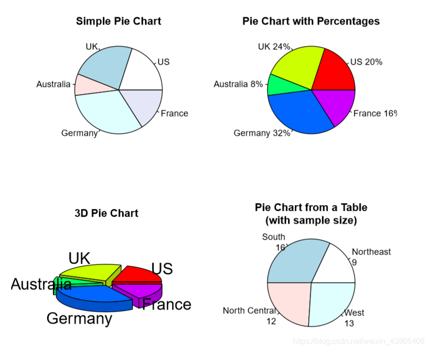
Pie Chart(饼图)
> library(plotrix)
> par(mfrow=c(2,2))
> slices <- c(10, 12,4, 16, 8)
> lbls <- c("US", "UK", "Australia", "Germany", "France")
> pie(slices, labels = lbls,main="Simple Pie Chart",edges=300,radius=1)
> pct <- round(slices/sum(slices)*100)
> lbls2 <- paste(lbls, " ", pct, "%", sep="")
> pie(slices, labels=lbls2, col=rainbow(length(lbls2)),
+     main="Pie Chart with Percentages",edges=300,radius=1)
> pie3D(slices, labels=lbls,explode=0.1,
+       main="3D Pie Chart ",edges=300,radius=1)
> mytable <- table(state.region)
> lbls3 <- paste(names(mytable), "\n", mytable, sep="")
> pie(mytable,labels=lbls3,
+     main="Pie Chart from a Table\n(with sample size)",
+     edges=300,radius=1)
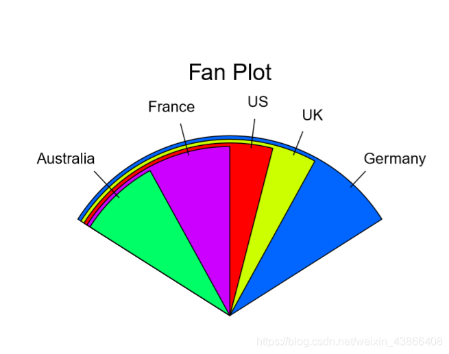
Fan Plot(扇形图)
> slices <- c(10, 12,4, 16, 8)
> lbls <- c("US", "UK", "Australia", "Germany", "France")
> fan.plot(slices, labels = lbls, main="Fan Plot")
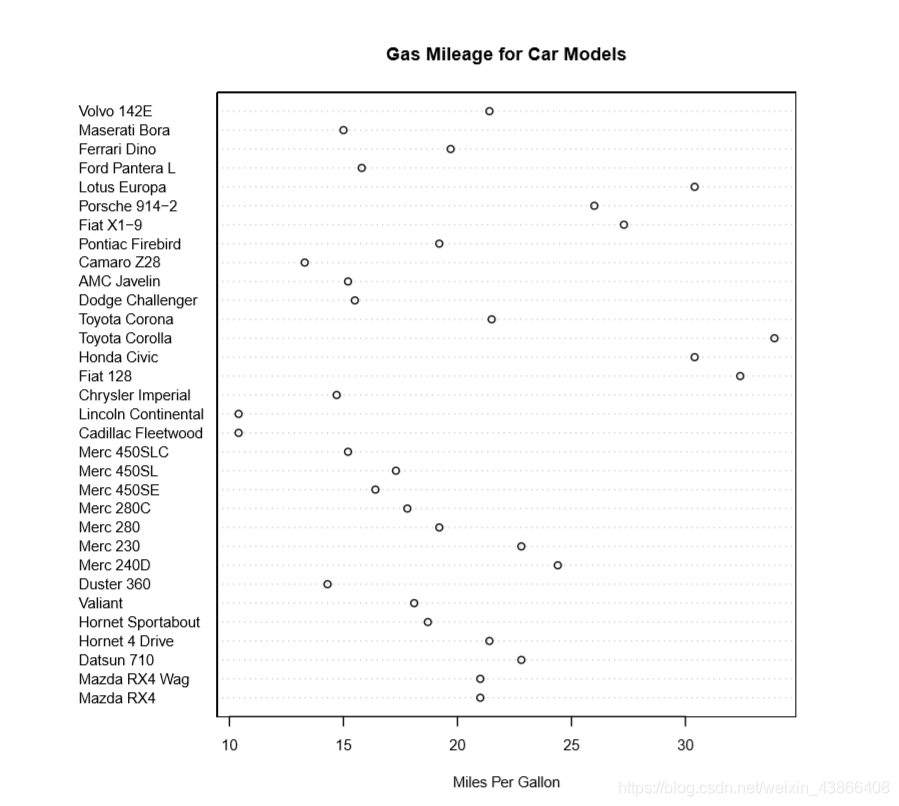
Dot Plot(点图)
> dotchart(mtcars$mpg,
+          labels=row.names(mtcars),cex=0.7,
+          main="Gas Mileage for Car Models",
+          xlab="Miles Per Gallon")
基础统计
描述统计
head(x)查看数据集,展示x的前几行(默认前6行),可以通过head(x,n=10)来显示前10行
> head(mtcars)
                   mpg cyl disp  hp drat
Mazda RX4         21.0   6  160 110 3.90
Mazda RX4 Wag     21.0   6  160 110 3.90
Datsun 710        22.8   4  108  93 3.85
Hornet 4 Drive    21.4   6  258 110 3.08
Hornet Sportabout 18.7   8  360 175 3.15
Valiant           18.1   6  225 105 2.76
                     wt  qsec vs am gear
Mazda RX4         2.620 16.46  0  1    4
Mazda RX4 Wag     2.875 17.02  0  1    4
Datsun 710        2.320 18.61  1  1    4
Hornet 4 Drive    3.215 19.44  1  0    3
Hornet Sportabout 3.440 17.02  0  0    3
Valiant           3.460 20.22  1  0    3
                  carb
Mazda RX4            4
Mazda RX4 Wag        4
Datsun 710           1
Hornet 4 Drive       1
Hornet Sportabout    2
Valiant              1
summary()获取描述性统计量,可以提供最小值、最大值、四分位数和数值型变量的均值,以及因子向量和逻辑型向量的频数统计等
> summary(mtcars)
      mpg             cyl
 Min.   :10.40   Min.   :4.000
 1st Qu.:15.43   1st Qu.:4.000
 Median :19.20   Median :6.000
 Mean   :20.09   Mean   :6.188
 3rd Qu.:22.80   3rd Qu.:8.000
 Max.   :33.90   Max.   :8.000
      disp             hp
 Min.   : 71.1   Min.   : 52.0
 1st Qu.:120.8   1st Qu.: 96.5
 Median :196.3   Median :123.0
 Mean   :230.7   Mean   :146.7
 3rd Qu.:326.0   3rd Qu.:180.0
 Max.   :472.0   Max.   :335.0
      drat             wt
 Min.   :2.760   Min.   :1.513
 1st Qu.:3.080   1st Qu.:2.581
 Median :3.695   Median :3.325
 Mean   :3.597   Mean   :3.217
 3rd Qu.:3.920   3rd Qu.:3.610
 Max.   :4.930   Max.   :5.424
      qsec             vs
 Min.   :14.50   Min.   :0.0000
 1st Qu.:16.89   1st Qu.:0.0000
 Median :17.71   Median :0.0000
 Mean   :17.85   Mean   :0.4375
 3rd Qu.:18.90   3rd Qu.:1.0000
 Max.   :22.90   Max.   :1.0000
       am              gear
 Min.   :0.0000   Min.   :3.000
 1st Qu.:0.0000   1st Qu.:3.000
 Median :0.0000   Median :4.000
 Mean   :0.4062   Mean   :3.688
 3rd Qu.:1.0000   3rd Qu.:4.000
 Max.   :1.0000   Max.   :5.000
      carb
 Min.   :1.000
 1st Qu.:2.000
 Median :2.000
 Mean   :2.812
 3rd Qu.:4.000
 Max.   :8.000
频率和列联表
table()可以展现变量的频率
> attach(mtcars)
> table(cyl)
cyl
 4  6  8
11  7 14
#cy1中4有11个,6有7个,8有14个
> summary(mpg)
   Min. 1st Qu.  Median    Mean 3rd Qu.
  10.40   15.43   19.20   20.09   22.80
   Max.
  33.90
#通过summary可以分析出mpg在[10,34]之间
#cut()可以讲区间划分
> table(cut(mpg,seq(10,34,by=2)))#10到34,2个一组

(10,12] (12,14] (14,16] (16,18] (18,20]
      2       1       7       3       5
(20,22] (22,24] (24,26] (26,28] (28,30]
      5       2       2       1       0
(30,32] (32,34]
      2       2
相关性
- cov(x,y):x和y间的协方差;如果x,y为矩阵或数据框,返回x和y各列的协方差
- var(x):向量x的样本方差;如果x是矩阵或数据框,协方差矩阵将被计算
- cor(x):如果x是矩阵或数据框,相关系数矩阵将被计算
求矩阵或数据框时cov=var
> states = state.x77[,1:6]
> cov(states)
              Population      Income
Population 19931683.7588 571229.7796
Income       571229.7796 377573.3061
Illiteracy      292.8680   -163.7020
Life Exp       -407.8425    280.6632
Murder         5663.5237   -521.8943
HS Grad       -3551.5096   3076.7690
             Illiteracy     Life Exp
Population  292.8679592 -407.8424612
Income     -163.7020408  280.6631837
Illiteracy    0.3715306   -0.4815122
Life Exp     -0.4815122    1.8020204
Murder        1.5817755   -3.8694804
HS Grad      -3.2354694    6.3126849
                Murder      HS Grad
Population 5663.523714 -3551.509551
Income     -521.894286  3076.768980
Illiteracy    1.581776    -3.235469
Life Exp     -3.869480     6.312685
Murder       13.627465   -14.549616
HS Grad     -14.549616    65.237894
> var(states)
              Population      Income
Population 19931683.7588 571229.7796
Income       571229.7796 377573.3061
Illiteracy      292.8680   -163.7020
Life Exp       -407.8425    280.6632
Murder         5663.5237   -521.8943
HS Grad       -3551.5096   3076.7690
             Illiteracy     Life Exp
Population  292.8679592 -407.8424612
Income     -163.7020408  280.6631837
Illiteracy    0.3715306   -0.4815122
Life Exp     -0.4815122    1.8020204
Murder        1.5817755   -3.8694804
HS Grad      -3.2354694    6.3126849
                Murder      HS Grad
Population 5663.523714 -3551.509551
Income     -521.894286  3076.768980
Illiteracy    1.581776    -3.235469
Life Exp     -3.869480     6.312685
Murder       13.627465   -14.549616
HS Grad     -14.549616    65.237894
> cor(states)
            Population     Income
Population  1.00000000  0.2082276
Income      0.20822756  1.0000000
Illiteracy  0.10762237 -0.4370752
Life Exp   -0.06805195  0.3402553
Murder      0.34364275 -0.2300776
HS Grad    -0.09848975  0.6199323
           Illiteracy    Life Exp
Population  0.1076224 -0.06805195
Income     -0.4370752  0.34025534
Illiteracy  1.0000000 -0.58847793
Life Exp   -0.5884779  1.00000000
Murder      0.7029752 -0.78084575
HS Grad    -0.6571886  0.58221620
               Murder     HS Grad
Population  0.3436428 -0.09848975
Income     -0.2300776  0.61993232
Illiteracy  0.7029752 -0.65718861
Life Exp   -0.7808458  0.58221620
Murder      1.0000000 -0.48797102
HS Grad    -0.4879710  1.00000000
T检验
> x = rnorm(100, mean = 10, sd = 1)#平均数为10,标准差为1
> y = rnorm(100, mean = 30, sd = 10)#平均数为30,标准差为10
> t.test(x, y, alt = "two.sided",paired=TRUE)

	Paired t-test

data:  x and y
t = -19.353, df = 99, p-value <
2.2e-16
alternative hypothesis: true difference in means is not equal to 0
95 percent confidence interval:
 -21.78096 -17.73004
sample estimates:
mean of the differences
               -19.7555
群体差异的非参数检验
> wilcox.test(x,y,alt="less")

	Wilcoxon rank sum test with
	continuity correction

data:  x and y
W = 294, p-value < 2.2e-16
alternative hypothesis: true location shift is less than 0
