
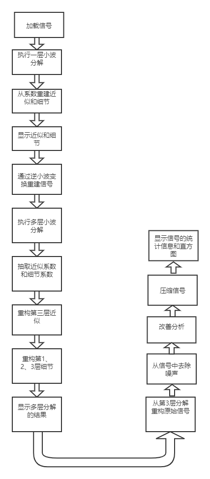
对信号进行一层分解
clc;
clear;
% 获取噪声信号
load('matlab.mat');
sig = M(1,1:1400);
SignalLength = length(sig);
%使用db1分解1层
 [cA1,cD1] = dwt(sig,'db1');
 %从系数 cA1 和 cD1 中构建一层近似A1 和细节 D1
 A1 = upcoef('a',cA1,'db1',1,SignalLength);
 D1 = upcoef('d',cD1,'db1',1,SignalLength);
   % %或
   % A1 = idwt(cA1,[],'db1',l_s);
   % D1 = idwt([],cD1,'db1',l_s);
 %显示近似和细节
 subplot(1,2,1); plot(A1); title('Approximation A1')
 subplot(1,2,2); plot(D1); title('Detail D1')
 %使用逆小波变换恢复信号
 A0 = idwt(cA1,cD1,'db1',SignalLength);
 err = max(abs(sig-A0))
对信号进行三层分解
[C,L] = wavedec(sig,3,'db1');%函数返回 3 层分解的各组分系数C(连接在一个向量里) ,向量 L 里返回的是各组分的长度。
 %抽取近似系数和细节系数
 %从 C 中抽取 3 层近似系数
 cA3 = appcoef(C,L,'db1',3);
 %从 C 中抽取 3、2、1 层细节系数
 [cD1,cD2,cD3] = detcoef(C,L,[1,2,3]);
 %或者
  %cD3 = detcoef(C,L,3);
  %cD2 = detcoef(C,L,2);
  %cD1 = detcoef(C,L,1);
 %重建 3 层近似和 1、2、3 层细节
 %从 C 中重建 3 层近似
 A3 = wrcoef('a',C,L,'db1',3);
 %从 C 中重建 1、2、3 层细节
 D1 = wrcoef('d',C,L,'db1',1);
 D2 = wrcoef('d',C,L,'db1',2);
 D3 = wrcoef('d',C,L,'db1',3);
 %显示多层分解的结果
 %显示 3 层分解的结果
 figure(2)
 subplot(2,2,1); plot(A3);
 title('Approximation A3')
 subplot(2,2,2); plot(D1);
 title('Detail D1')
 subplot(2,2,3); plot(D2);
 title('Detail D2')
 subplot(2,2,4); plot(D3);
 title('Detail D3')
 %从 3 层分解中重建原始信号
 A0 = waverec(C,L,'db1');
 err = max(abs(sig-A0))
 %  我们注意到连续的近似随着越来越多的高频信息从信号中滤除,
 % 噪声变得越
 % 来越少。 3 层近似与原始信号对比会发现变得很干净。对比近似和原始信号,如下
 figure(3)
 subplot(2,1,1);plot(sig);title('Original'); axis off
 subplot(2,1,2);plot(A3);title('Level 3 Approximation');axis off
这篇博客是参考百度文档上一位大佬写的,这是数据和文章的链接
链接:https://pan.baidu.com/s/19_jazLnyBuperh7ME5NG8Q
提取码:aonu