利用自相关函数对分析音频的周期变化

摘要

一个音频文件音调随着时间的变化，每个微小时间段的频率是不一样的，也就是说周期是不一样的，通过求声音信号的关于时间的自相关函数得到其周期改变，进而得出其频率规律。

结果及分析

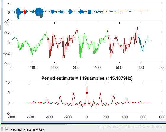
按任意键移动时间区间，分析不同时间段的信号周期。图一是原始信号，图二是提取时间段的信号频谱图，图三是自相关函数图。

• 可以由图三看到，信号并不是有一个简单的周期函数加入噪声形成的，应该有多个周期函数。
• 假设可以把最高的那几个峰近似看成同一个周期函数的自相关函数，那么他的周期是160~170ms左右，就是频率在6.3 ~ 5.9HZ这样子。
  

拓展

更多相关函数的内容请看这里。

完整代码

测试音频下载链接在这里，也可以用歌曲、录音如mp3格式的文件测试，不过会由于文件较大而比较慢。

%% Using Autocorrelation to track the local period of a signal
% This code is used as part of a youtube video demonstration 
% See http://youtube.com/ddorran
%
% Code available at https://dadorran.wordpress.com       
%
% The following wav file can be downloaded from 
%       https://www.dropbox.com/s/3y25abf1xuqpizj/speech_demo.wav
%% speech analysis example
 
[ip fs] = audioread('speech_demo.wav');
max_expected_period = round(1/50*fs);
min_expected_period = round(1/200*fs);
frame_len = 2*max_expected_period;
 
for k = 1 : length(ip)/frame_len -1;
    range = (k-1)*frame_len + 1:k*frame_len;
    frame = ip(range);
     
    %show the input in blue and the selected frame in red
    plot(ip);
    set(gca, 'xtick',[],'position',[ 0.05  0.82   0.91  0.13])
    hold on;
    temp_sig = ones(size(ip))*NaN;
    temp_sig(range) = frame;
    plot(temp_sig,'r');
    hold off
     
    %use xcorr to determine the local period of the frame
    [rxx lag] = xcorr(frame, frame);
    subplot(3,1,3)
    plot(lag, rxx,'r')
    rxx(find(rxx < 0)) = 0; %set any negative correlation values to zero
    center_peak_width = find(rxx(frame_len:end) == 0 ,1); %find first zero after center
    %center of rxx is located at length(frame)+1
    rxx(frame_len-center_peak_width : frame_len+center_peak_width  ) = min(rxx);
%     hold on
%     plot(lag, rxx,'g');
%     hold off
    [max_val loc] = max(rxx);
    period = abs(loc - length(frame)+1); 
     
    title(['Period estimate = ' num2str(period) 'samples (' num2str(fs/period) 'Hz)']);
    set(gca, 'position', [ 0.05  0.07    0.91  0.25])
     
    [max_val max_loc] = max(frame);
    num_cycles_in_frame = ceil(frame_len/period);
    test_start_positions = max_loc-(period*[-num_cycles_in_frame:num_cycles_in_frame]);
    index = find(test_start_positions > 0,1, 'last');
    start_position = test_start_positions(index);
    colours = 'rg';
     
    subplot(3,1,2)
    plot(frame);
     
    set(gca, 'position',[ 0.05 0.47 0.91 0.33])
    pause
    for g = 1 : num_cycles_in_frame
        if(start_position+period*(g) <= frame_len && period > min_expected_period)
            cycle_seg = ones(1, frame_len)*NaN;
            cycle_seg(start_position+period*(g-1):start_position+period*(g))  =...
                            frame(start_position+period*(g-1):start_position+period*(g));
            hold on
             
            plot(cycle_seg,colours(mod(g, length(colours))+1)) %plot one of the available colors
            hold off
        end
    end
    pause
end
 
%% synthesise a periodic signal to use as a basic demo
fs = 500;
T = 1/fs;
N = 250; % desired length of signal
t = [0:N-1]*T; %time vector 
f1 = 8; f2=f1*2; 
x = sin(2*pi*f1*t-pi/2) + sin(2*pi*f2*t);
plot(t, x)
ylabel('Amplitude')
xlabel('Time (seconds)')
title('Synthesised Signal');
 
%% Determine the autocorrelation function
[rxx lags] = xcorr(x,x);
figure
plot(lags, rxx)
xlabel('Lag')
ylabel('Correlation Measure')
title('Auto-correlation Function')
 
%% Illustrate the auto correlation process
%function available from https://dadorran.wordpress.com
illustrate_xcorr(x,x) 
 
%% Identify most prominent peaks
% Most prominent peak will be at the center of the correlation function
first_peak_loc = length(x) + 1;
 
% Lots of possible ways to identify second prominent peak. Am going to use a crude approach
% relying on some assumed prior knowledge of the signal. Am going to assume
% that the signal has a minimum possible period of .06 seconds = 30 samples;
min_period_in_samples = 30; 
half_min = min_period_in_samples/2 ;
 
seq = rxx;
seq(first_peak_loc-half_min: first_peak_loc+half_min) = min(seq);
plot(rxx,'rx');
hold on
plot(seq)
 
[max_val second_peak_loc] = max(seq);
period_in_samples =  abs(second_peak_loc -first_peak_loc)
period = period_in_samples*T
fundamental_frequency = 1/period
 
%% Autocorrelation of a noisy signal 
x2 = x + randn(1, length(x))*0.2;
plot(x2)
ylabel('Amplitude')
xlabel('Time (seconds)')
title('Noisy Synthesised Signal');
 
[rxx2 lags] = xcorr(x2,x2);
figure
plot(lags, rxx2)
xlabel('Lag')
ylabel('Correlation Measure')
title('Auto-correlation Function')
 
%% Autocorrelation technique can be problematic!
% Consider the following signal
f1 = 8; f2=f1*2; 
x3 = sin(2*pi*f1*t) + 5*sin(2*pi*f2*t);
plot(t, x3)
ylabel('Amplitude')
xlabel('Time (seconds)')
title('Synthesised Signal');
 
[rxx3 lags] = xcorr(x3,x3,'unbiased');
figure
plot(lags, rxx3)
xlabel('Lag')
ylabel('Correlation Measure')
title('Auto-correlation Function')
 
seq = rxx3;
seq(first_peak_loc-half_min: first_peak_loc+half_min) = min(seq);
plot(seq)
 
[max_val second_peak_loc] = max(seq);
period_in_samples =  abs(second_peak_loc -first_peak_loc)