无人驾驶12：路径规划，生成路径曲线

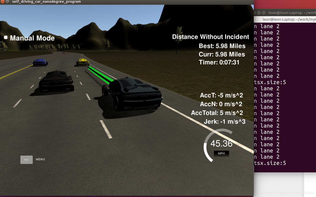
优达学城的第7个项目实现：https://github.com/luteresa/P7-Path-Planning.git

运动规划问题：

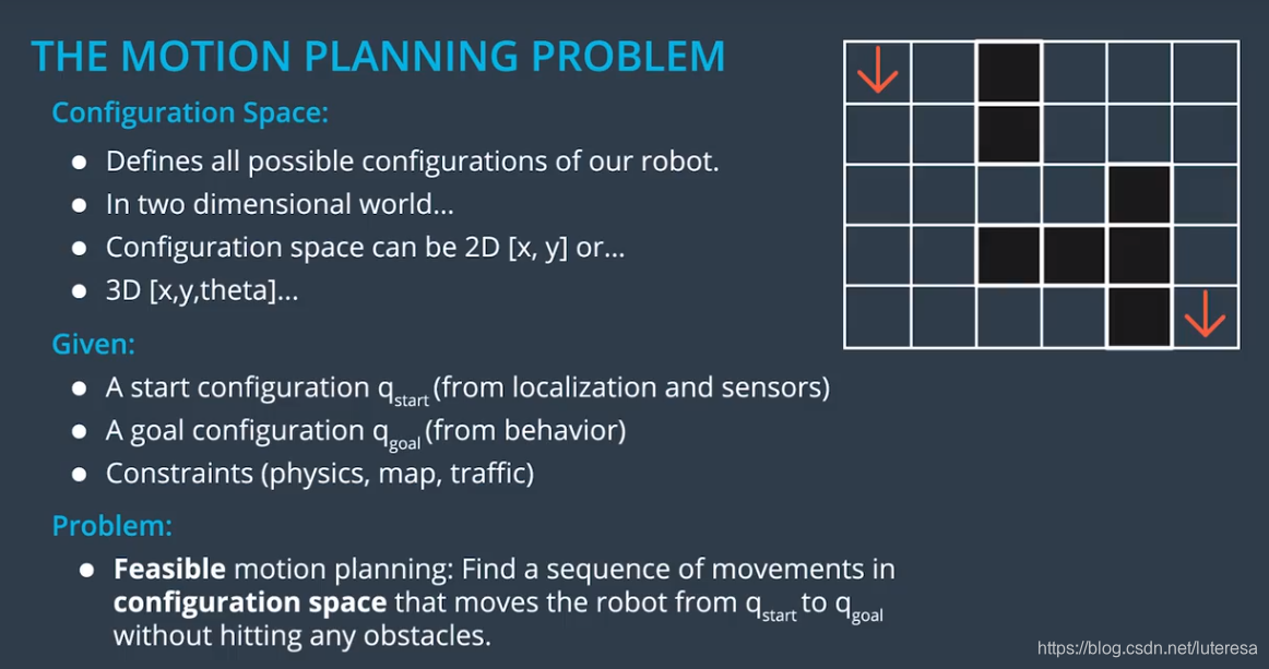
配置空间

配置空间：定义机器人的所有可能配置，一般在二维空间中，定义为[x,y, theat]，即二维坐标加方向。

运动规划：

就是根据初始配置(由定位模块传感器获得)，目的配置(由行为规划模块获得)，在一定的限制条件下(车辆属性，交通法规)，结合预测模块(提供有关障碍区域随时间演进的信息)，在配置空间中，生成一个可执行的运动序列(纳入了其他车辆及行人考量)。

这些运动(可转化为车辆的最终指令，比如刹车，油门，转向)将驱动机器人，从开始配置移动到目标配置，过程中会绕开障碍物，

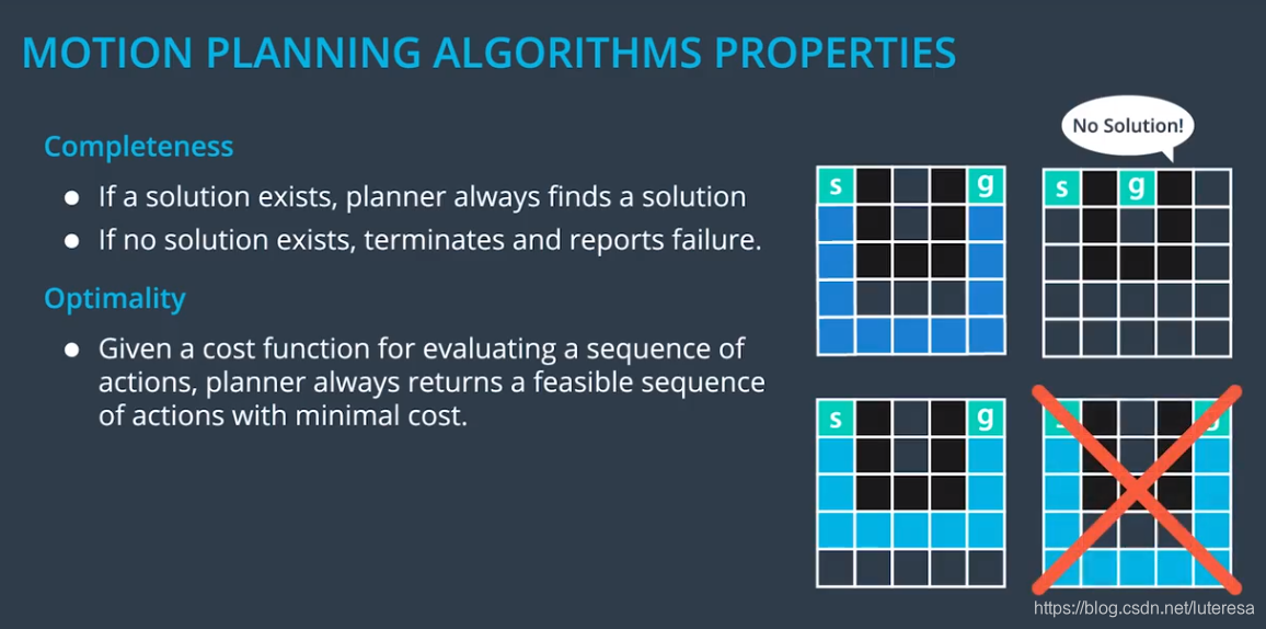
讨论规划算法时，常需要考虑两个重要因素，完整性和最优性

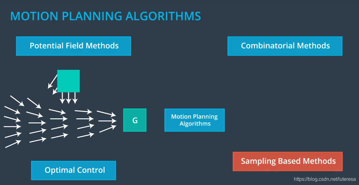
运动规划算法有很多种，包括

组合法：将自由空间分成小块，然后将这些原子元素链接起来，解决运动规划问题；这种方法与我们直觉相符，去发现最初的近似解；但当环境规模扩大后，这种方法表现不佳；

位势场算法：是反馈算法，每个障碍物会产生一种反重力场，这使车辆不会去靠近它们。比如算法轨迹会绕过行人和自行车；
位势场算法的主要问题是，有时候它会把我们带入局部极小值中。难以找到最合适解；

最优控制法：通过算法来生成控制PoD，使用动态模型，为车辆，最初配置和最终配置建模，概算法需要我们生成一系列的输入，比如转向和减速，这些输入会把我们从开始配置带到最终配置。在此过程中，算法会优化与控制输入，车辆配置等相关的成本函数。比如最小汽油消耗。这种算法有多种实现方式，大部分都基于数值优化法；

但是要把所有与其他车辆相关的限制都很好地纳入考量，还要使算法很快地的得出结果，是相当困难的。

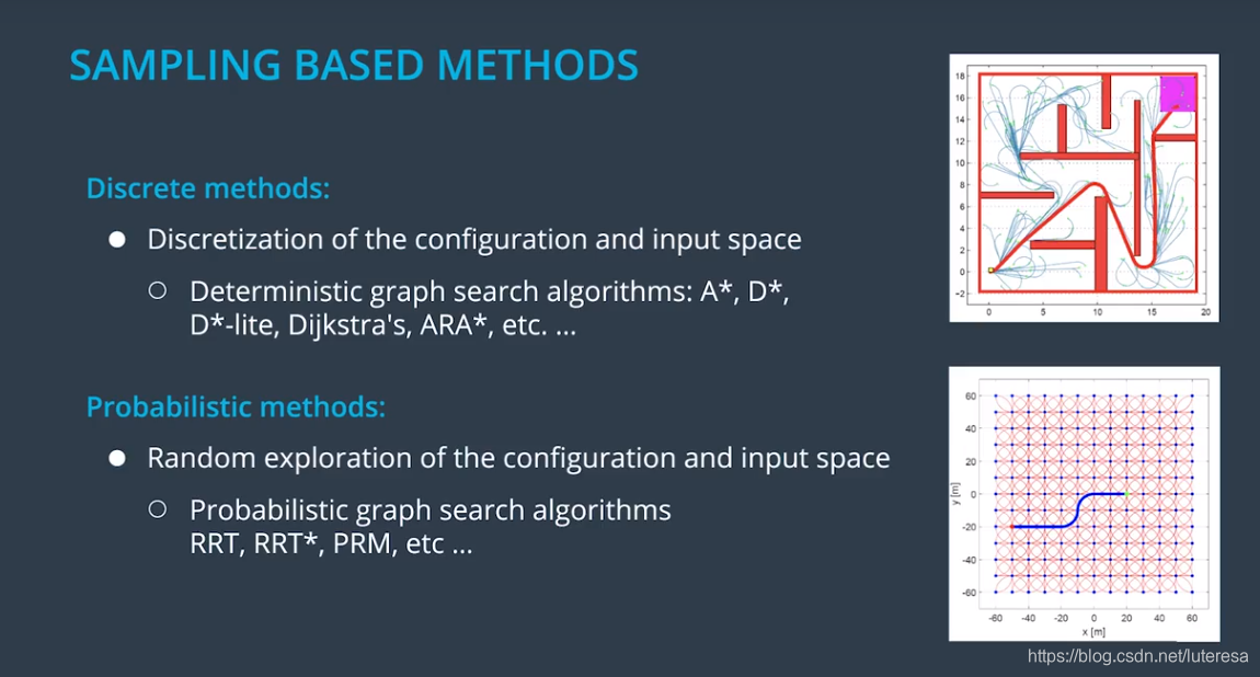
抽样算法：使用一个基于碰撞检测的模块，该模块探测自由空间，测试是否一个配置在其中会发生碰撞，不同于组合法和最优控制法(这两种方法均需要分析整个环境)，抽样法不需要检测所有自由空间，便可以发现一条路径，搜索过的路径保存在一个图结构中，然后使用图搜索算法例如 $D^\star 或者A^\star$来搜索。

有两种方法可以认定是基于抽样的，

离散法：它依赖于构造良好的辅助集合或者输入，比如覆盖在我们配置空间上的一张格子图；

概率统计法：它依赖连续配置空间的概率样本，待探索的可能配置或者状态集，可能是无穷多的，这让这类算法具有一种不错的性质，那就是它们是概率完整的，并且有时候概率的优化，意味着它们最终会找出一个解来，前提是给予足够的计算时间。

$Hybrid A^\star$

1.混合 $A^\star$的更新方程

(假设无人车为自行人模型)

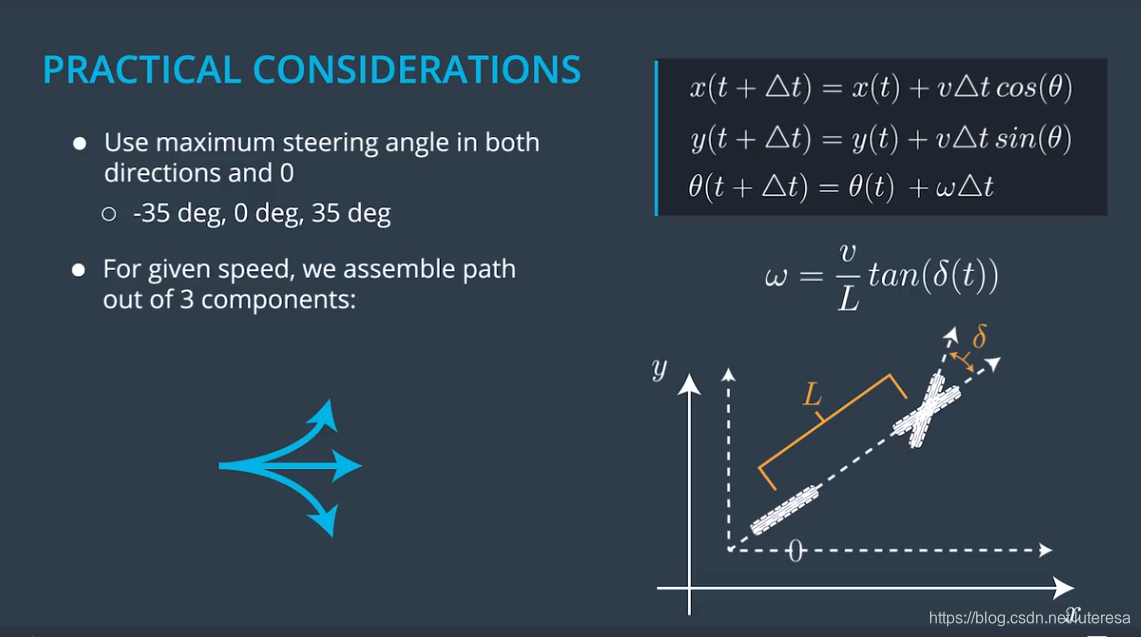
这个方程对于绝大部分具有X，Y域的配置空间是通用的。

无人车应用中， $\omega$是个受限值，因为无人车不可能围绕Z周无限转动(扫地机器人可以)。

假设最大转向角（左右均）为 $35^o$，可以用3种新的基本运动来扩展搜索树，搜索迷宫效果

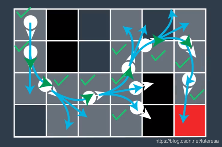
去掉多余信息，得到一条平滑的可驾驶曲线。

1.不是最优的，也不一定是最平滑的。；

2.有时候找不出存在解(为了实现连续，丢弃了部分网格扩展方向的完整性)；
为了解决该问题，可以给搜索空间添加第三维，即朝向，这样不会过早关闭实际有解的配置空间。

和标准 $A^\star$相比，混合 $A^\star$牺牲了少许完整性和优化性，但是确保了可驾驶性。

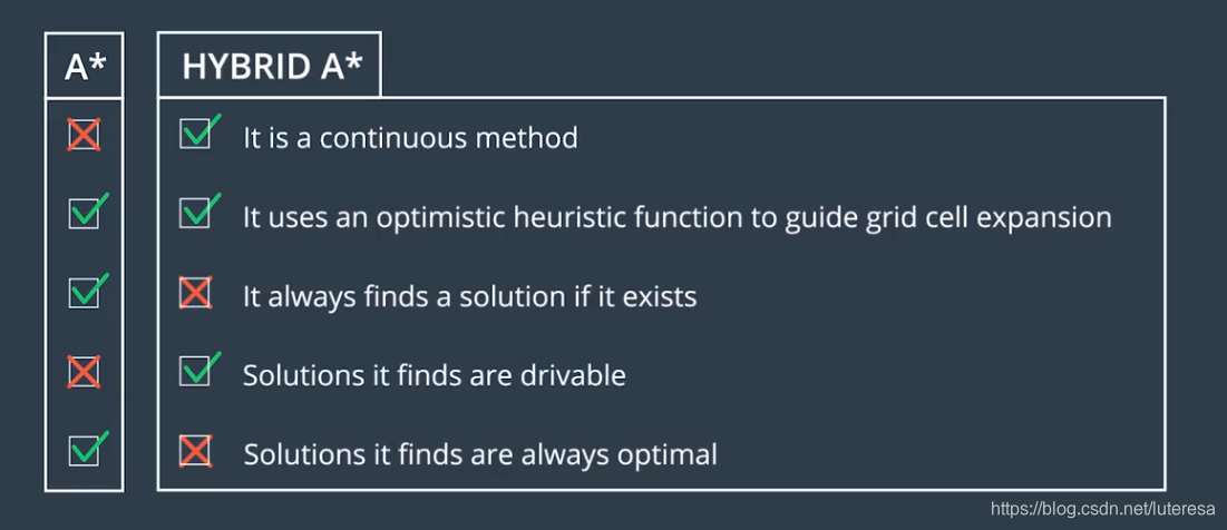
而在实际应用中，混合 $A^\star$效率极高，而且几乎每次都可以找到不错的路径。

2. $Hybrid A^\star$的启发函数

The paper Junior: The Stanford Entry in the Urban Challenge is a good read overall, but Section 6.3 - Free Form Navigation is especially good and goes into detail about how the Stanford team thought about heuristics for their Hybrid A* algorithm (which they tended to use in parking lots).

伪代码实现：

def expand(state, goal):
    next_states = []
    for delta in range(-35, 40, 5): 
        # Create a trajectory with delta as the steering angle using 
        # the bicycle model:

        # ---Begin bicycle model---
        delta_rad = deg_to_rad(delta)
        omega = SPEED/LENGTH * tan(delta_rad)
        next_x = state.x + SPEED * cos(theta)
        next_y = state.y + SPEED * sin(theta)
        next_theta = normalize(state.theta + omega)
        # ---End bicycle model-----

        next_g = state.g + 1
        next_f = next_g + heuristic(next_x, next_y, goal)

        # Create a new State object with all of the "next" values.
        state = State(next_x, next_y, next_theta, next_g, next_f)
        next_states.append(state)

    return next_states

def search(grid, start, goal):
    # The opened array keeps track of the stack of States objects we are 
    # searching through.
    opened = []
    # 3D array of zeros with dimensions:
    # (NUM_THETA_CELLS, grid x size, grid y size).
    closed = [[[0 for x in range(grid[0])] for y in range(len(grid))] 
        for cell in range(NUM_THETA_CELLS)]
    # 3D array with same dimensions. Will be filled with State() objects 
    # to keep track of the path through the grid. 
    came_from = [[[0 for x in range(grid[0])] for y in range(len(grid))] 
        for cell in range(NUM_THETA_CELLS)]

    # Create new state object to start the search with.
    x = start.x
    y = start.y
    theta = start.theta
    g = 0
    f = heuristic(start.x, start.y, goal)
    state = State(x, y, theta, 0, f)
    opened.append(state)

    # The range from 0 to 2pi has been discretized into NUM_THETA_CELLS cells. 
    # Here, theta_to_stack_number returns the cell that theta belongs to. 
    # Smaller thetas (close to 0 when normalized  into the range from 0 to 
    # 2pi) have lower stack numbers, and larger thetas (close to 2pi when 
    # normalized) have larger stack numbers.
    stack_num = theta_to_stack_number(state.theta)
    closed[stack_num][index(state.x)][index(state.y)] = 1

    # Store our starting state. For other states, we will store the previous 
    # state in the path, but the starting state has no previous.
    came_from[stack_num][index(state.x)][index(state.y)] = state

    # While there are still states to explore:
    while opened:
        # Sort the states by f-value and start search using the state with the 
        # lowest f-value. This is crucial to the A* algorithm; the f-value 
        # improves search efficiency by indicating where to look first.
        opened.sort(key=lambda state:state.f)
        current = opened.pop(0)

        # Check if the x and y coordinates are in the same grid cell 
        # as the goal. (Note: The idx function returns the grid index for 
        # a given coordinate.)
        if (idx(current.x) == goal[0]) and (idx(current.y) == goal.y):
            # If so, the trajectory has reached the goal.
            return path

        # Otherwise, expand the current state to get a list of possible 
        # next states.
        next_states = expand(current, goal)
        for next_s in next_states:
            # If we have expanded outside the grid, skip this next_s.
            if next_s is not in the grid:
                continue
            # Otherwise, check that we haven't already visited this cell and
            # that there is not an obstacle in the grid there.
            stack_num = theta_to_stack_number(next_s.theta)
            if closed[stack_num][idx(next_s.x)][idx(next_s.y)] == 0 
                and grid[idx(next_s.x)][idx(next_s.y)] == 0:
                # The state can be added to the opened stack.
                opened.append(next_s)
                # The stack_number, idx(next_s.x), idx(next_s.y) tuple 
                # has now been visited, so it can be closed.
                closed[stack_num][idx(next_s.x)][idx(next_s.y)] = 1
                # The next_s came from the current state, and is recorded.
                came_from[stack_num][idx(next_s.x)][idx(next_s.y)] = current

代码实现：

HBF::maze_path HBF::search(vector< vector<int> > &grid, vector<double> &start, 
                           vector<int> &goal) {
  // Working Implementation of breadth first search. Does NOT use a heuristic
  //   and as a result this is pretty inefficient. Try modifying this algorithm 
  //   into hybrid A* by adding heuristics appropriately.

  /**
   * TODO: Add heuristics and convert this function into hybrid A*
   */
  vector<vector<vector<int>>> closed(
    NUM_THETA_CELLS, vector<vector<int>>(grid[0].size(), vector<int>(grid.size())));
  vector<vector<vector<maze_s>>> came_from(
    NUM_THETA_CELLS, vector<vector<maze_s>>(grid[0].size(), vector<maze_s>(grid.size())));
  double theta = start[2];
  int stack = theta_to_stack_number(theta);
  int g = 0;

  maze_s state;
  state.g = g;
  state.x = start[0];
  state.y = start[1];
  state.theta = theta;
  state.f = g + heuristic(state.x, state.y, goal);

  closed[stack][idx(state.x)][idx(state.y)] = 1;
  came_from[stack][idx(state.x)][idx(state.y)] = state;
  int total_closed = 1;
  vector<maze_s> opened = {state};
  bool finished = false;
  while(!opened.empty()) {
  	sort(opened.begin(), opened.end(), compare_maze_s);
    maze_s current = opened[0]; //grab first elment
    opened.erase(opened.begin()); //pop first element

    int x = current.x;
    int y = current.y;

    if(idx(x) == goal[0] && idx(y) == goal[1]) {
      std::cout << "found path to goal in " << total_closed << " expansions" 
                << std::endl;
      maze_path path;
      path.came_from = came_from;
      path.closed = closed;
      path.final = current;

      return path;
    }

    vector<maze_s> next_state = expand(current, goal);//扩展多个可运动的方向

    for(int i = 0; i < next_state.size(); ++i) {
      int g2 = next_state[i].g;
      double x2 = next_state[i].x;
      double y2 = next_state[i].y;
      double theta2 = next_state[i].theta;

      if((x2 < 0 || x2 >= grid.size()) || (y2 < 0 || y2 >= grid[0].size())) {
        // invalid cell
        continue;
      }
      //stack2范围是多少？
      int stack2 = theta_to_stack_number(theta2);

      if(closed[stack2][idx(x2)][idx(y2)] == 0 && grid[idx(x2)][idx(y2)] == 0) {
        opened.push_back(next_state[i]);
        closed[stack2][idx(x2)][idx(y2)] = 1;
        came_from[stack2][idx(x2)][idx(y2)] = current;
        ++total_closed;
      }
    }
  }

  std::cout << "no valid path." << std::endl;
  HBF::maze_path path;
  path.came_from = came_from;
  path.closed = closed;
  path.final = state;

  return path;
}

环境分类

此算法是非结构化环境中，路径探寻的最佳算法之一。

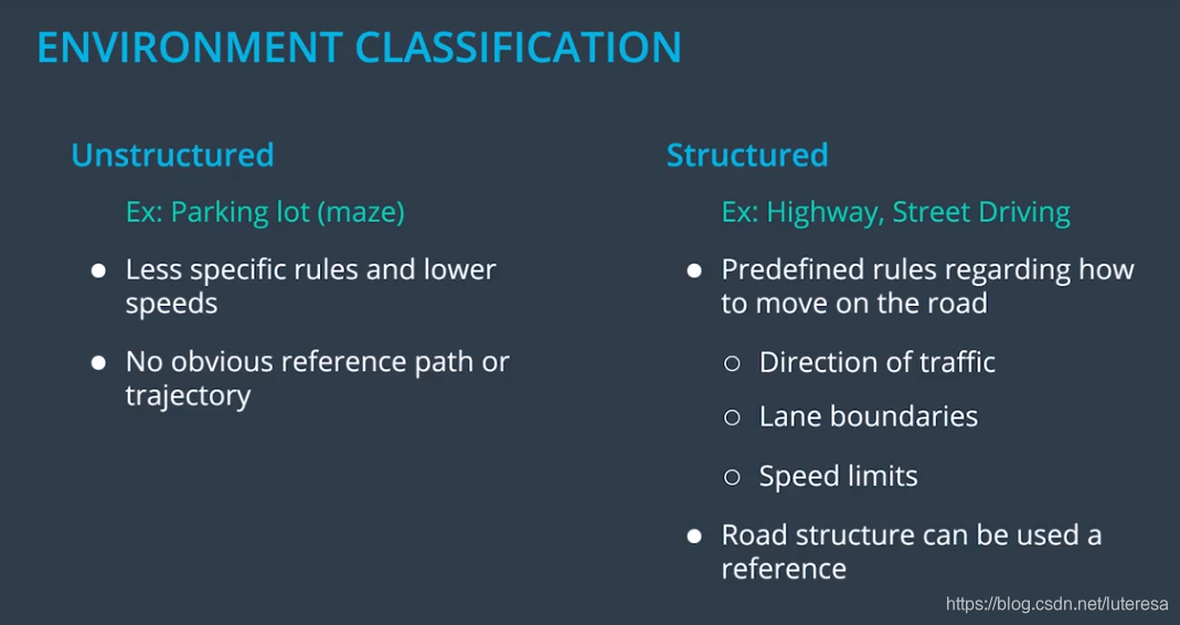
非结构化场景：应用实例有停车场和迷宫等，特点是驾驶规则限制少，速度低，与高速公路以及城市环境殊为不同，这种环境里并不存在明显的参考路径（也就是哪种车辆90%时间都在上面行驶的路径），因为这种环境中，情况随时在变化。

结构化场景：相比而言，高速公路和街道是相当结构化的环境，所有的驾驶都在预定义规则的限制下进行，而我们的驾驶也可按照某些规则进行，如车辆行驶方向、车道边界、速度限制等。这些规则对车辆行驶加以限制，当我们生成运动轨迹时，也必须满足所有这些规则。

一种在无规则下的最佳算法，如果不能有效利用这些规则，则不适合这种结构化环境。

而对于高速公路这种结构化的环境，我们可以有效利用环境规则，比如以车道线为参考。下面学习一种适合高速公路的轨迹生成算法。

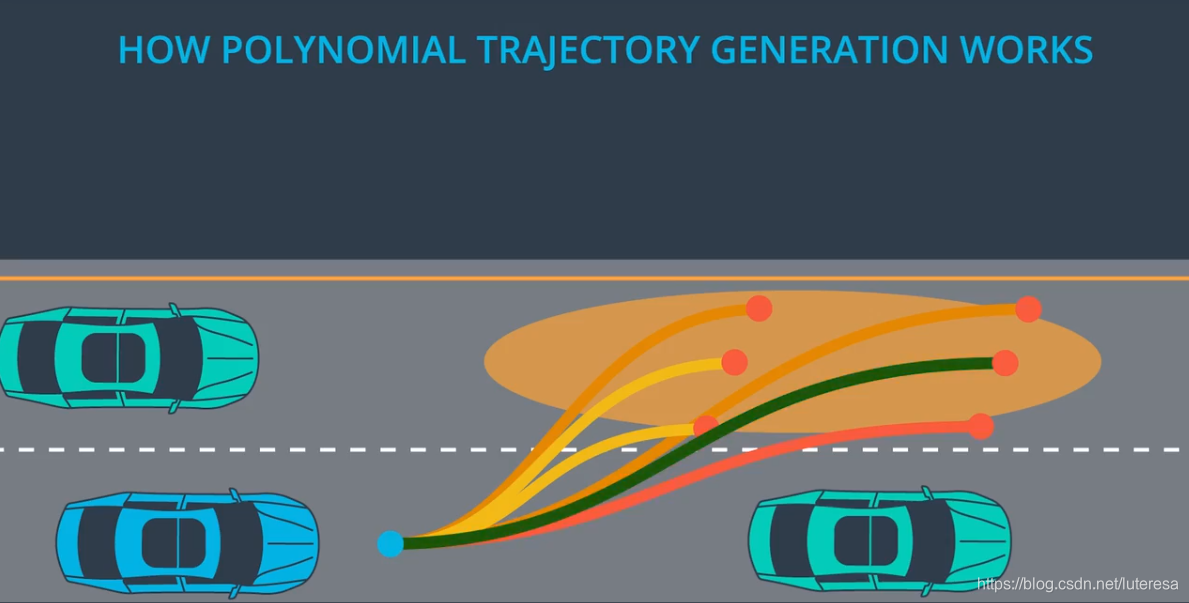
多项式轨迹法(适用高速环境)

Frenet 坐标系, s, d, t

用Frenet坐标，可以简化车辆运动模型，比如高速路上的一个超车场景

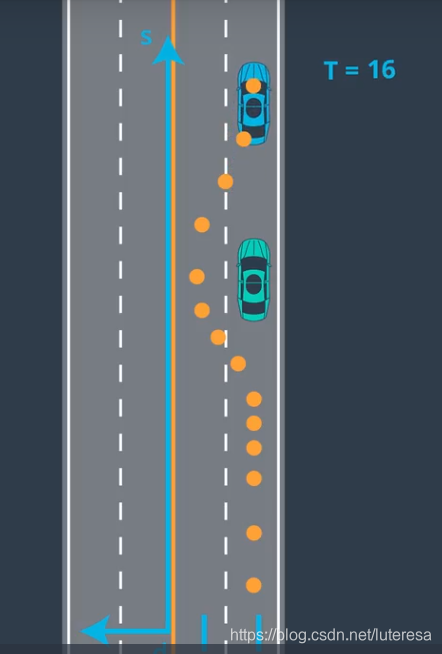
该场景实际上还忽略了一个因素，时间t，因为高速上的环境是动态的，随时可能有车周边经过。

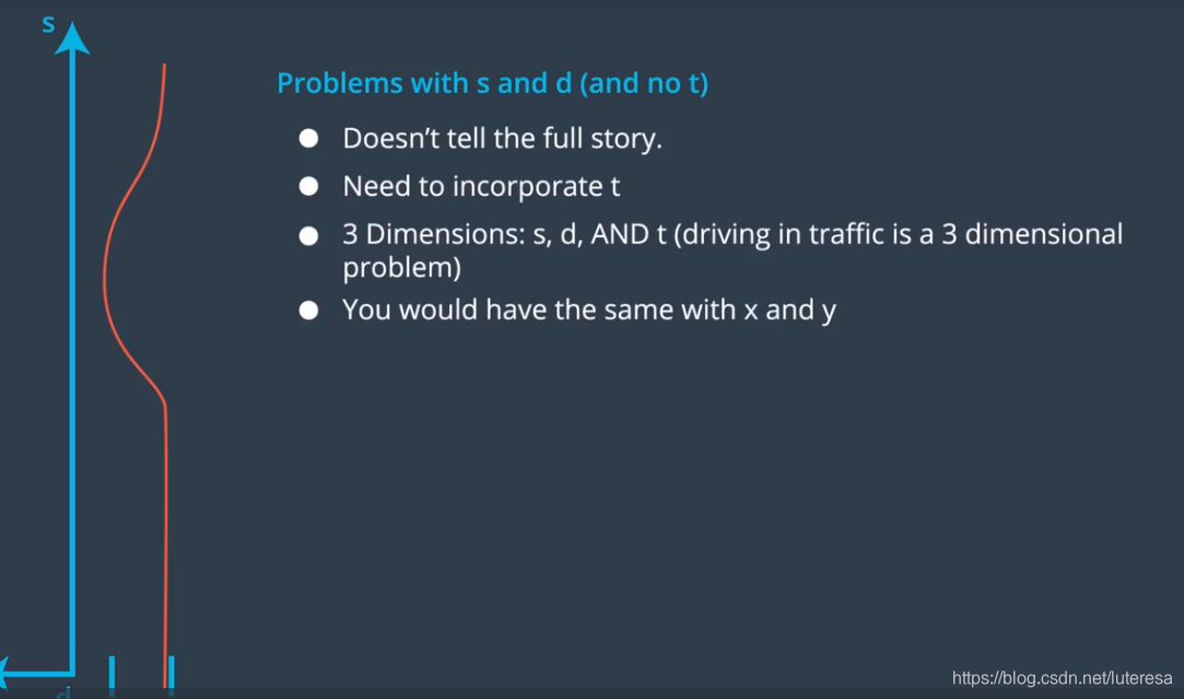
考虑三维场景(因场景是随机的，必须考虑时间因素)

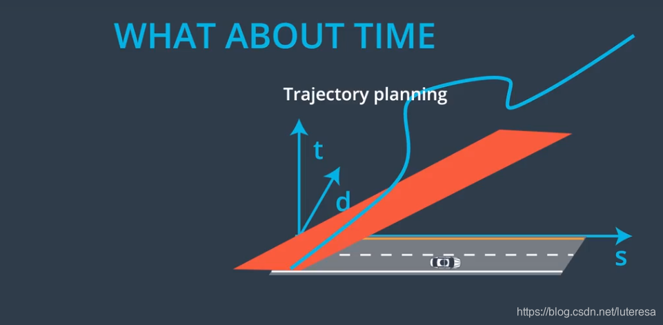
将三维场景分解为两个独立的二维模型, s/t, d/t

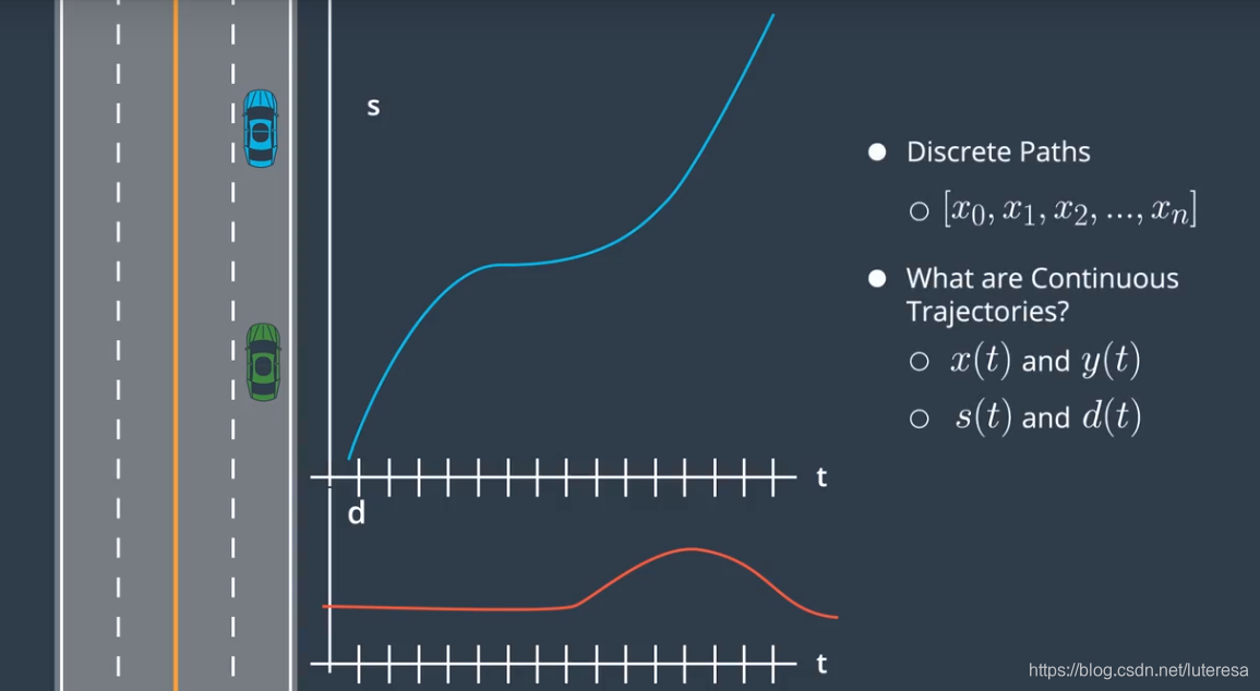
Structured Trajectory Generation Overview

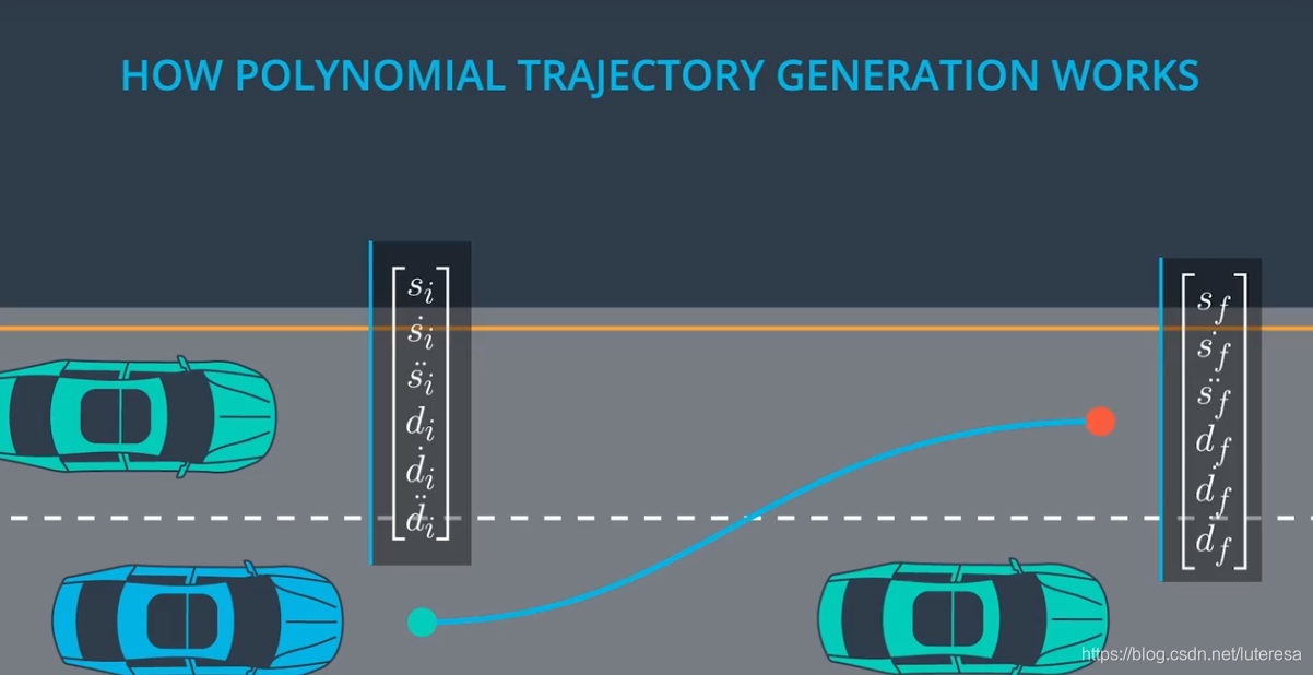
我们的目标是生成连续的轨迹，轨迹是一个函数，在任一时间点上，该函数可以求得一辆车的一个配置.

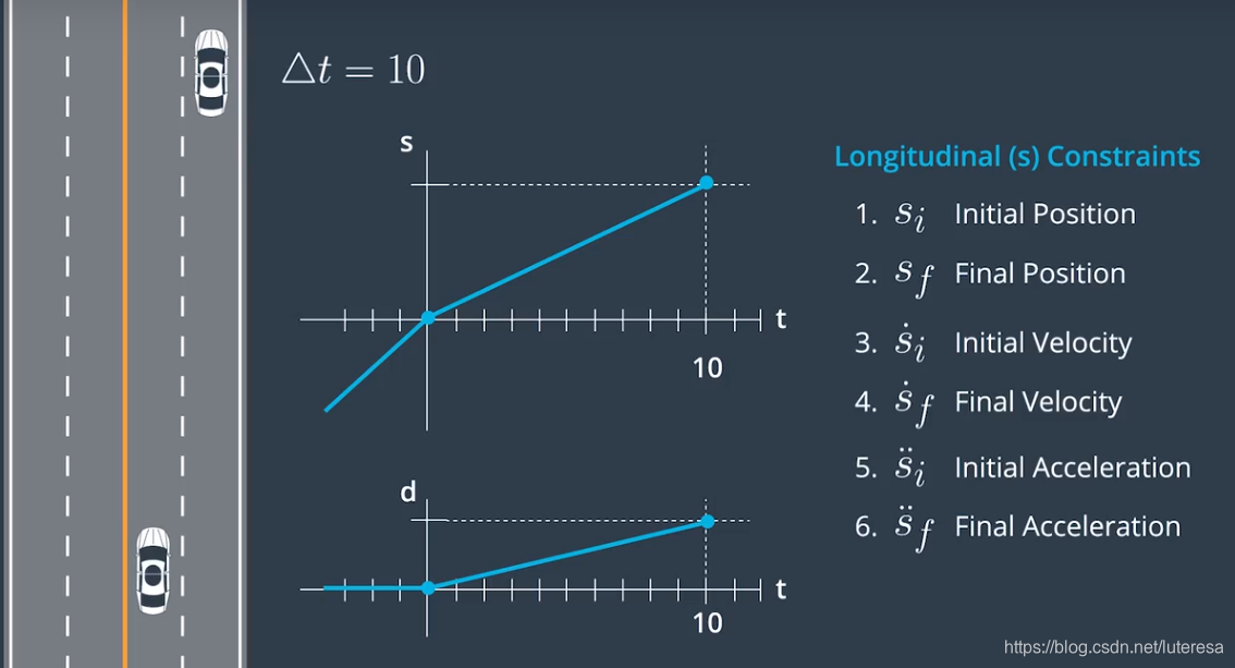
比如下场景，汽车在高速路上匀速行驶，10S后需要驶出高速，即已知当前状态(位置，速度，加速度)，终点状态，以及时间，拟合出最佳的连续曲线。

拟合的曲线，既要考虑连续性，还要考虑平滑性，否则车辆会给人不舒适感甚至出现危险。

很明显，引起不舒适感的因素是加速度的变化率（颠簸）。

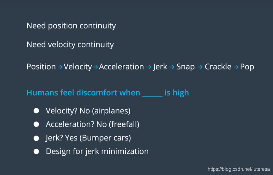
到这里，问题转化为，拟合曲线，并且加速度变化率最小(最舒适)，即jerk最小化

jerk minimizing轨迹

按上面分析问题简化为，在单个维度，s或者d，找出能够使得Jerk(t)最小的轨迹.

Takahashi等人已经证明：任何Jerk最优化问题中的解都可以用一个5次多项式来表示：

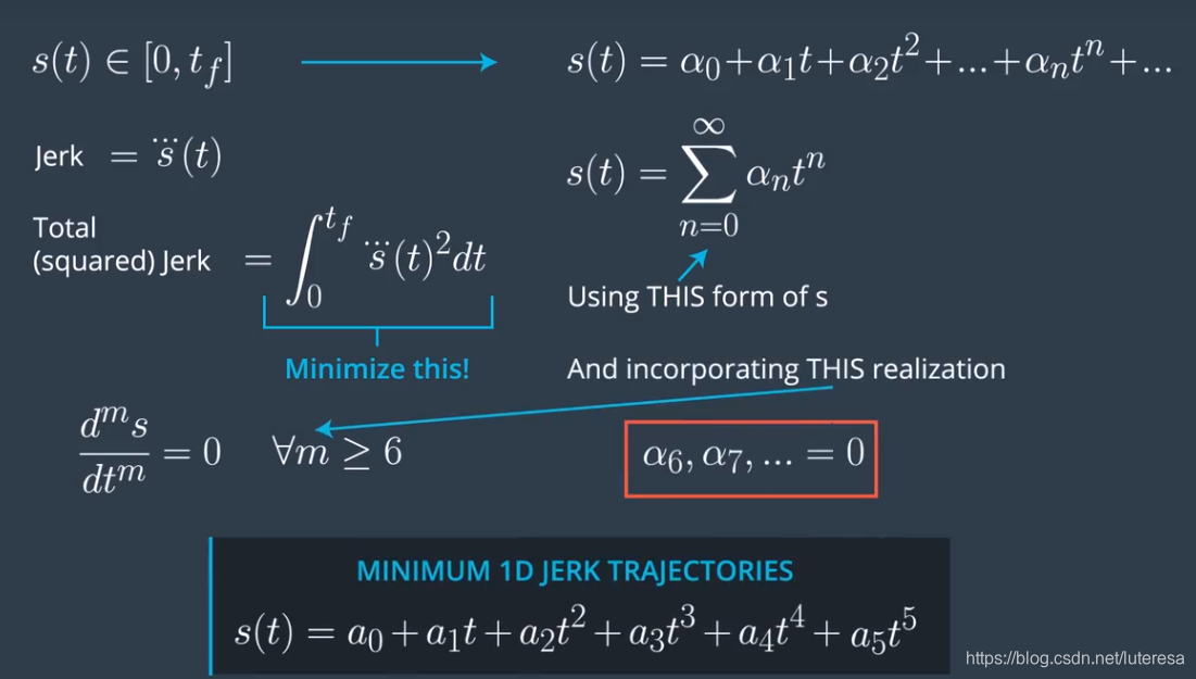
问题转化为，根据边界条件，求5次多项式，对应有6个可调参数，6个边界条件

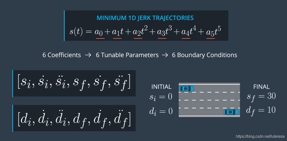
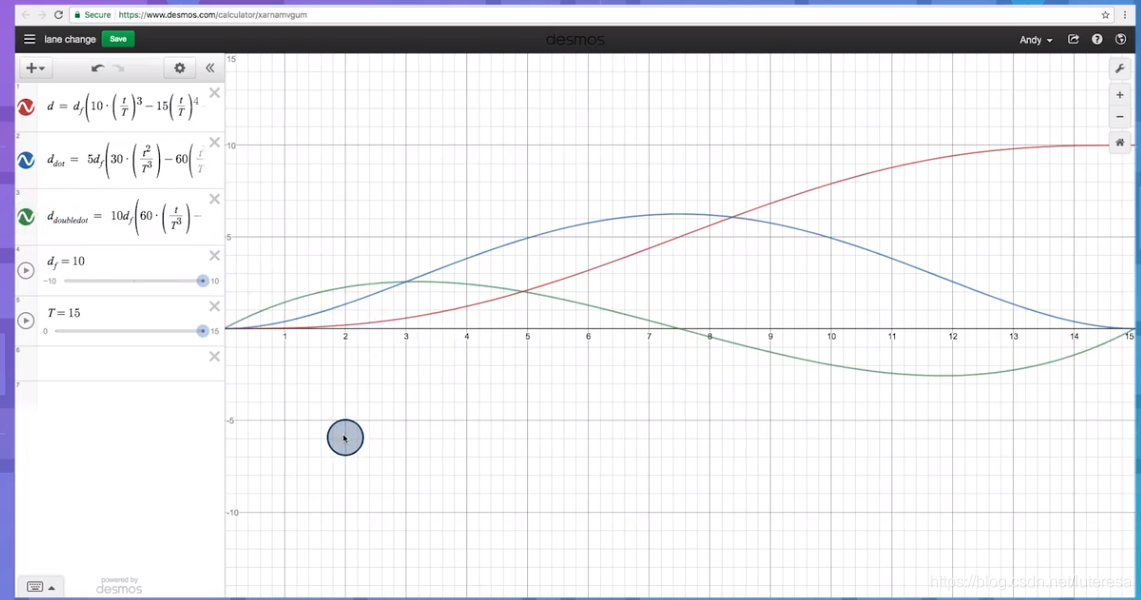
假设横轴d的初始速度/加速度，最终速度/加速度均为0,运动曲线如下：

求Jerk系数方法：

根据运动学公式，对s(t)1次求导得到速度，2次求导得到加速度，公式如下：

$s(t) = \alpha_0 + \alpha_1t + \alpha_2t^2 + \alpha_3t^3 + \alpha_4t^4 + \alpha_5^5$

$\dot s(t) = \alpha_1 + 2\alpha_2t + 3\alpha_3t^2 + 4\alpha_4t^3 + 5\alpha_5^4$

$\ddot s(t) = 2\alpha_2 + 6\alpha_3t + 12\alpha_4t^2 + 20\alpha_5^3$

对初始边界条件， $t_i=0$:
$s_i = s(0) = \alpha_0$

$\dot{s_i} = \dot{s_i}(0) = \alpha_1$

$\ddot{s_i} = \ddot{s_i}(0) = 2\alpha_2$

这样，就只剩下3个未知系数：

$s(t) = s_i + \dot{s_i}t + \frac{\ddot{s_i}}{2}t^2 + \alpha_3t^3 + \alpha_4t^4 + \alpha_5t^5s(t)$

$\dot{s}(t) = \dot{s_i} + \ddot{s_i}t + 3 \alpha_3t^2 + 4\alpha_4t^3 + 5\alpha_5t^4$

$\ddot{s}(t) = \ddot{s_i} + 6 \alpha_3t + 12\alpha_4t^2 + 20\alpha_5t^3$

方程改写为：
$s(t) = \alpha_3t^3 + \alpha_4t^4 + \alpha_5^5 + C_1$

$\dot s(t) = 3\alpha_3t^2 + 4\alpha_4t^3 + 5\alpha_5^4 + C_2$

$\ddot s(t) = 6\alpha_3t + 12\alpha_4t^2 + 20\alpha_5^3 + C_3$

当t不等于0时，

$s(t_f) = \alpha_3t^3 + \alpha_4t^4 + \alpha_5^5 + C_1$

$\dot s(t_f) = 3\alpha_3t^2 + 4\alpha_4t^3 + 5\alpha_5^4 + C_2$

$\ddot s(t_f) = 6\alpha_3t + 12\alpha_4t^2 + 20\alpha_5^3 + C_3$

写成矩阵形式：

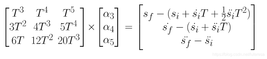
根据最终配置空间值和时间，就可以求出所有系数。

实现代码：

vector<double> JMT(vector<double> &start, vector<double> &end, double T) {
  /**
   * Calculate the Jerk Minimizing Trajectory that connects the initial state
   * to the final state in time T.
   *
   * @param start - the vehicles start location given as a length three array
   *   corresponding to initial values of [s, s_dot, s_double_dot]
   * @param end - the desired end state for vehicle. Like "start" this is a
   *   length three array.
   * @param T - The duration, in seconds, over which this maneuver should occur.
   *
   * @output an array of length 6, each value corresponding to a coefficent in 
   *   the polynomial:
   *   s(t) = a_0 + a_1 * t + a_2 * t**2 + a_3 * t**3 + a_4 * t**4 + a_5 * t**5
   *
   * EXAMPLE
   *   > JMT([0, 10, 0], [10, 10, 0], 1)
   *     [0.0, 10.0, 0.0, 0.0, 0.0, 0.0]
   */
	MatrixXd A = MatrixXd(3,3);
	auto T2 = T*T;
  	auto T3 = T2*T;
	auto T4 = T2*T2;
	auto T5 = T3*T2;
	A << T3,T4,T5,
		3*T2,4*T3,5*T4,
		6*T, 12*T2,20*T3;
  	MatrixXd B = MatrixXd(3,1);
  	B << end[0] - (start[0] + start[1]*T + 0.5*start[2]*T2),
  	end[1] - (start[1] + start[2]*T),
  	end[2] - start[2];

	MatrixXd 
Ai = A.inverse();

	MatrixXd C = Ai*B;

  	vector<double> result = {start[0],start[1],0.5*start[2]};

	for (int i = 0; i < C.size(); i++) {
		result.push_back(C.data()[i]);
	}

	return result;
}

同样，在横轴上也可以求出其6个参数。

即，在初始状态，目标状态都已知的情况下，给定一个时间t，就可以可到一个连续，平滑的曲线。

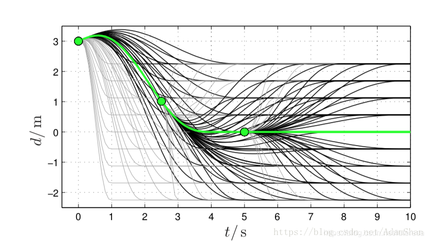
如何选择最优

按上面的方法，对每个不同的目标配置空间，或时间T，都可以生成不同的Jerk轨迹，

那么如何选择最优轨迹，需要考虑哪些限制条件呢？

设计代价函数：

$C_d = k_jJ_t(d(t)) + k_tT + k_d d1^2$

$k_jJ_t(d(t))$: 惩罚Jerk较大的备选轨迹；

$k_tT$: 制动应当迅速，时间段；

$k_d d1^2$: 目标状态不应偏离道路中心线太远；

其中 $k_j, k_t,k_d$是这三个惩罚项的比例系数，也叫权重值，它们的大小决定是代价函数更偏向哪一方便优化。

以上损失函数仅适用于高速场景，在极端低速情况下，车辆的制动能力是不完整的，不能再将d设计为t的五次多项式，损失函数也会有所不同，

但是这种基于优先采样轨迹的思路，以及通过优化损失函数搜索最优轨迹的方法原理是相通的。

在纵向上，优化场景大致分三类:

跟车

汇流和停车

车速保持

在高速公路等应用场景中，目标配置中并不需要考虑目标位置（即 $s_1$ ），所以初始目标配置仍然是 $(s_0,\dot{s_0},\ddot{s_0})$，目标配置变成 $\dot{s_1},\ddot{s_1}$，损失函数为：

$C_s = k_jJ_t(s(t)) + k_tT + k_{\dot{s}}(\dot{s_1} - \dot{s_c})^2$

其中 $s_c$ 是我们想要保持的纵向速度，第三个惩罚项的引入实际上是为了让目标配置中的纵向速度尽可能接近设定速度，该情景下的目标配置集为：
$[\dot{s_1}, \ddot{s_1}, T]_{ij} = [[\dot{s_c} + \Delta\dot{s_i}], 0, T_j]$

即优化过程中的可变参数为 $\Delta\dot{s_i}$ 和 $T_j$ ，同样，也可以通过设置 $\Delta T$ 和 $\Delta \dot s$ 来设置轨迹采样的密度，从而获得一个有限的纵向轨迹集合：

以上分别讨论了横向和纵向最优轨迹搜索方法，在应用中也可以将两个方差合并为一个：
$C_{total} = k_{lat}C_d + k_{lon}C_s$
这样，就可以通过最小化 $C_{total}$得到优化轨迹集合，不仅可以得到“最优”估计参数，还可以得到“次优”，“次次优”轨迹等。

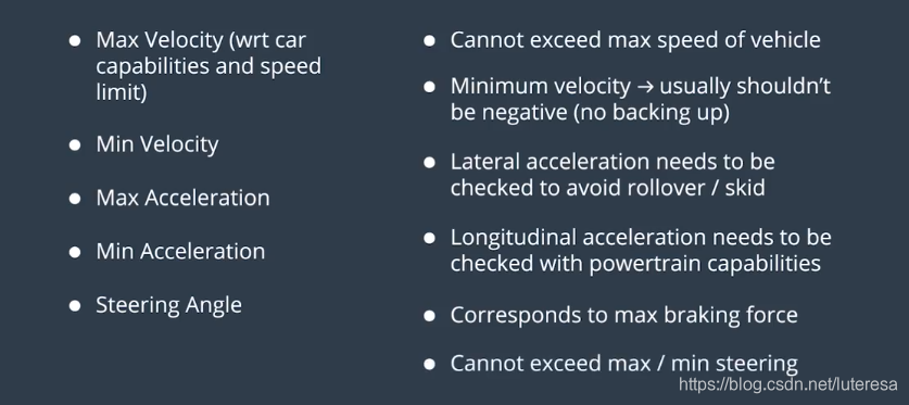
可行性检测

我们设计的损失函数，并没有包括障碍物规避的相关惩罚，也没有最大速度，最大加速度和最大曲率等控制约束限制。

每考虑这些的主要原因是，使得损失函数设计非常复杂。

基于Frenet坐标系的方法，是将这些因素的考量独立出来，在完成优化轨迹以后进行。

对所有完成的轨迹做一次可行性检测，过滤不符合约束条件，或碰到障碍物的轨迹。

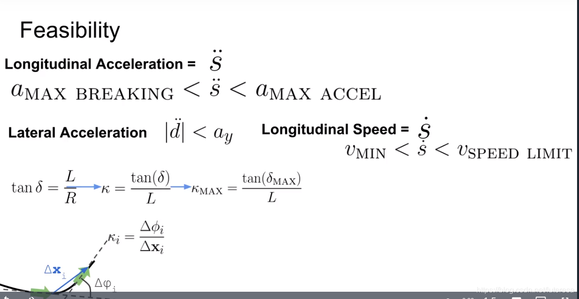
检查内容一般有：

s方向上的速度是否超过设定的最大限速

s方向的加速度是否超过设定的最大加速度

轨迹的曲率是否超过最大曲率

轨迹是否会引起碰撞（事故）

障碍物规避，又与行为预测有关联，也可在预测部分就规避掉，两者都是一个复杂的课题。

Optimal Trajectory Generation For Dynamic Street Scenarios In A Frenet Frame

小结：

以上学习了好几种轨迹生成算法，在解决无人驾驶汽车遇到的所有情况时，没有哪种方法可以说是最佳方法；

现实中的无人车会使用若干种方法，依情况而定，在停车场，可能使用混合方法，在车流量不大的高速上，可能使用多项式轨迹生成法；

同时也许会使用别的方法来应对其他情况，比如分叉路口，车流密集道路等。

Additional Resources on Path Planning

Indoors
Intention-Net: Integrating Planning and Deep Learning for Goal-Directed Autonomous Navigation by S. W. Gao, et. al.

Abstract: How can a delivery robot navigate reliably to a destination in a new office building, with minimal prior information? To tackle this challenge, this paper introduces a two-level hierarchical approach, which integrates model-free deep learning and model-based path planning. At the low level, a neural-network motion controller, called the intention-net, is trained end-to-end to provide robust local navigation. The intention-net maps images from a single monocular camera and “intentions” directly to robot controls. At the high level, a path planner uses a crude map, e.g., a 2-D floor plan, to compute a path from the robot’s current location to the goal. The planned path provides intentions to the intention-net. Preliminary experiments suggest that the learned motion controller is robust against perceptual uncertainty and by integrating with a path planner, it generalizes effectively to new environments and goals.

City Navigation

Learning to Navigate in Cities Without a Map by P. Mirowski, et. al.

Abstract: Navigating through unstructured environments is a basic capability of intelligent creatures, and thus is of fundamental interest in the study and development of artificial intelligence. Long-range navigation is a complex cognitive task that relies on developing an internal representation of space, grounded by recognizable landmarks and robust visual processing, that can simultaneously support continuous self-localization (“I am here”) and a representation of the goal (“I am going there”). Building upon recent research that applies deep reinforcement learning to maze navigation problems, we present an end-to-end deep reinforcement learning approach that can be applied on a city scale. […] We present an interactive navigation environment that uses Google StreetView for its photographic content and worldwide coverage, and demonstrate that our learning method allows agents to learn to navigate multiple cities and to traverse to target destinations that may be kilometers away. […]

Intersections

A Look at Motion Planning for Autonomous Vehicles at an Intersection by S. Krishnan, et. al.

Abstract: Autonomous Vehicles are currently being tested in a variety of scenarios. As we move towards Autonomous Vehicles, how should intersections look? To answer that question, we break down an intersection management into the different conundrums and scenarios involved in the trajectory planning and current approaches to solve them. Then, a brief analysis of current works in autonomous intersection is conducted. With a critical eye, we try to delve into the discrepancies of existing solutions while presenting some critical and important factors that have been addressed. Furthermore, open issues that have to be addressed are also emphasized. We also try to answer the question of how to benchmark intersection management algorithms by providing some factors that impact autonomous navigation at intersection.

Planning in Traffic with Deep Reinforcement Learning

DeepTraffic: Crowdsourced Hyperparameter Tuning of Deep Reinforcement Learning Systems for Multi-Agent Dense Traffic Navigation by L. Fridman, J. Terwilliger and B. Jenik

Abstract: We present a traffic simulation named DeepTraffic where the planning systems for a subset of the vehicles are handled by a neural network as part of a model-free, off-policy reinforcement learning process. The primary goal of DeepTraffic is to make the hands-on study of deep reinforcement learning accessible to thousands of students, educators, and researchers in order to inspire and fuel the exploration and evaluation of deep Q-learning network variants and hyperparameter configurations through large-scale, open competition. This paper investigates the crowd-sourced hyperparameter tuning of the policy network that resulted from the first iteration of the DeepTraffic competition where thousands of participants actively searched through the hyperparameter space.