【RCNN系列】Faster RCNN目标检测模型

上篇文章阐述了Fast RCNN网络模型，介于Faster RCNN属于RCNN系列的经典模型，以及是目前项目暂使用的目标检测模型，本篇文章会结合论文以及tensorflow版本的代码实现详细的阐述该模型。【可能篇幅会很长，毕竟经典模型，慎重】

Faster RCNN论文：https://arxiv.org/abs/1506.01497

Faster RCNN论文翻译：https://alvinzhu.xyz/2017/10/12/faster-r-cnn/

一、概述

Faster RCNN（Fast Regions with CNN features）相对于Fast RCNN是一种更快速的目标检测模型。相对于Fast RCNN 66%的mAP，其不仅在缩减训练、测试时长的情况下，也提高了准确度。(主干网络VGG16, mAP70.7%, resnet101 mAP75%)。

【Faster RCNN目标检测模型提出了与RCNN、SPPNet、Fast RCNN(选择搜索算法)不一样的区域提取模式RPN网络模型，该模型优化了Fast RCNN在时间上的性能瓶颈。RPN网络和检测网络共享全图的卷积，并且可以在每个位置同时预测目标边界和objectness得分。】

二、Faster RCNN网络模型

Faster RCNN物体检测系统由三个模块组成：

特征提取网络
RPN网络
区域归一化、物体分类以及边框回归

1、特征提取网络

Faster RCNN提取特征的主干网络可以是VGG16的前13层，13Conv+4次池化。

2、RPN网络

RPN(Region Proposal Network) 区域提案网络，较之Fast RCNN单独的Selective Search选择搜索算法提取候选框，将候选框提取融合到整个网络中。

区域提案网络（Region Proposal Network, RPN），它和检测网络共享全图的卷积特征，使得区域提案几乎不花时间。RPN是一个全卷积网络，在每个位置同时预测目标边界和objectness得分。RPN是端到端训练的，生成高质量区域提案框，用于Fast R-CNN来检测。我们通过共享其卷积特征进一步将RPN和Fast R-CNN合并到一个网络中。使用最近流行的神经网络术语“注意力”机制，RPN模块将某块anchor box打分比较高，则后面的网络对其进行训练。

说到RPN网络，则需要提到锚点（anchor）和边框回归。

【Anchor】

【原理】滑动窗口在特征图上滑动，每经过一个anchor点就会产生3种尺度和3种长宽比K(K = 9)个提案框。每个提案框包含2类信息，一个是该提案框是否包含物体，二是该提案框的坐标编码。每个anchor在cls分类层（softmax二分类）会输出2*K个分类得分（每个anchor box 前景背景得分），在reg回归层(线性回归)会产生4K个输出(每个anchor box都有4个坐标)，对于大小为H*W的卷积特征映射，总共会产生W*H*K个anchor boxes。

【属性】使用Anchor提取候选区域具有一些属性：

1、平移不变性，即图片中物体的也会被其它的anchor的anchor box框选到；

2、基于参照多个尺度和纵横比设计的锚点，可以简单地使用单尺度图像上的卷积特征，无需额外的成本来缩放尺寸。

(a) 图像金字塔 (b)卷积金字塔 (d)参考框金字塔(RPN)

【边框回归】

【摘要】RCNN、Fast RCNN、Faster RCNN都需要用到边界框回归来预测物体的目标检测框。边界框回归要做的就是利用某种映射关系，使得候选目标框经过映射后更加接近于真实目标框。

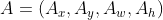
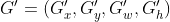
Anchor与预测

Anchro边框、预测边框、真实边框

  【原理】

设Anchor的坐标预测边框G'的坐标真实边框G的坐标

$A=(A_x, A_y, A_w, A_h)$    $G'=(G'_x, G'_y, G'_w, G'_h)$ $G=(G_x,G_y,G_w,G_h)$

边框回归就是寻找一种变换 $f$ , 使得

$f(A_x,A_y,A_w,A_h) = (G'_x,G'_y,G'_w,G'_h)$ $(G'_x,G'_y,G'_w,G'_h) \approx (G_x,G_y,G_w,G_h)$

A和G'之间的关系：

【平移】：

$G'_x=A_w \cdot d_x(A)+A_x; G'_y=A_w \cdot d_y(A)+A_y$

  【缩放】：

$G'_w = A_w\cdot exp(d_w(A)); G'_h = A_h\cdot exp(d_h(A))$

边框回归需要【学习】的就是：

   $d_x(A),d_y(A),d_w(A),d_h(A)$

【当anchor A与GT相差较小时(在进行线性回归时会筛选anchor和gt IOU在一定范围内的anchor，这也就保证了anchor与GT的相差不会很大)，可以认为这种变换时一种线性变换，则可以用线性回归建模。即Y = WX】

【Y = WX 】输入的X是 cnn feature map,定义为 $\phi$ ，那么：

$d_*(A) = W_*^T\cdot \phi (A)$

【 $d_*(A)$ 表示的是Anchor的坐标和预测的贴近真实框的预测的坐标的线性关系，而Anchor的坐标和真实框的坐标的线性关系是怎么样呢，这两个关系又是什么关系呢，是否是学习与被学习的关系。】

根据上面Anchor和预测G’的坐标关系可知Anchor坐标和GT坐标的关系是：

   $t_x(A)=(G_x-A_x)/A_w;t_y(A)=(G_y-A_y)/A_h;$

$t_w(A)=log(G_w/A_w);t_h(A)=log(G_h/A_h)$

【通过上面的公式，可得知 $d_*(A)$ 就是要拟合(变成) $t_*(A)$ 】， $d_*(A) = W_*^T\cdot \phi (A)$ ，所以整个线性回归其实就是学习一组

   $W_*[W_x,W_y,W_w,W_y]$

优化目标为：

$w_*=argmin_w_*\sum _i^N(t_*^i - w_*^T\iphi (A^i))^{2}+\lambda ||w_*||^{2}$    $\lambda ||w_*||^{2}$ 是正则项防止过拟合

Smooth_L1损失函数：

$Loss=\sum _i^N|t_*^i - w_*^T\iphi (A^i)|$

【Propoasl层】

Proposal层输入三个参数，anchor box前景、背景打分，以及anchor box偏移关系和im_Info（原图信息），那该层的作用：

对于所有的anchor boxes，结合输入的偏移关系，进行回归，也就是将偏移叠加到anchor boxes上修正原始anchor boxes，

利用anchor box的打分情况和NMS筛选出一定数目的偏移后的anchor boxes。

【RPN】

RPN主要作用是生成区域提案，里面设计了分类和边框回归。

【分类】：anchor产生的anchor box 通过softmax二分类网络判断该区域提案为前景(包含目标)和背景（不包含）的得分。基于该分类的得分，可以作为筛选过多anchor的手段。

【边框回归】：

通过anchor和真实边框的关系（平移、缩放） $t_*(A)$ ，来优化anchor和预测边框（其实在这里预测边框是不存在，是anchor叠加回归输出的偏移）的关系 $d_*(A)$ ，边框回归输出的不是坐标而是一种关系，也就是anchor和预测边框之间的偏移情况，在Propoasl层才将回归输出的偏移叠加到anchor坐标上，来修正anchor坐标，这也是对anchor的第一次修正，后面还有第二次修正。

边框回归的偏移关系 $d_*(A) = W_*^T\cdot \phi (A)$ ，输入是特征向量，所以边框回归要学习的是参数 $W_*^[W_x,W_y,W_w,W_h]$ ，

也就是通过不同目标的特征，分别学习针对该目标特征对应的 $W_*^[W_x,W_y,W_w,W_h]$ 参数，也就是该参数的维度应该是包含可以检测的所有物体类别数目。

【输出】

RPN网络最终得到训练（256）、测试（300）对应的anchor box的前景、后景得分情况，以及该anchor box的坐标。

3、区域归一化、物体分类以及边框回归

区域归一化、物体分类以及边框回归这里的结构就和Fast RCNN基本一致了，在此就不做阐述了。

三、Faster RCNN代码解析

该图来自：https://www.cnblogs.com/darkknightzh/p/10043864.html

下面就结合上面的图，针对代码一步一步分析：

代码的主体结构在_build_network函数里。

    def _build_network(self, is_training=True):
        """
        该函数总体流程：
            1、通过分类网络（vgg16、resnet）得到特征net_cov
            2、将net_cov送入rpn网络得到候选区域anchors，训练则筛选出2000个anchor，测试则筛选出 
               300个anchors，在进一步筛选出256个anchors用于分类
            3、将256个anchors进行rois_pooling操作得到pool5的7*7的特征图
            4、将pool5通过两个fc得到fc7得到21维的cls_score和21*4的bbox_pred
        :param is_training:
        :return:
        """
        # 是否使用截断正态分布
        if cfg.TRAIN.TRUNCATED:
            initializer = tf.truncated_normal_initializer(mean=0.0, stddev=0.01)
            initializer_bbox = tf.truncated_normal_initializer(mean=0.0, stddev=0.001)
        else:
            initializer = tf.random_normal_initializer(mean=0.0, stddev=0.01)
            initializer_bbox = tf.random_normal_initializer(mean=0.0, stddev=0.001)
        # 分类网络处理生成特征图
        net_conv = self._image_to_head(is_training)

        with tf.variable_scope(self._scope, self._scope):
            # 为特征图创建anchors（特征图是原图/16，anchors的个数是特征图像素数*9，而每个 
            #anchor是在原图上的坐标，该函数返回anchors的坐标矩阵和anchors数量 ）
            self._anchor_component()
            # RPN网络对特征进行处理，最终得到256（训练）个anchors对应类别以及坐标或者300（测 
            #试）个anchors对应类别以及坐标
            rois = self._region_proposal(net_conv, is_training, initializer)
            # roi pooling层将特征向量resize到指定大小
            if cfg.POOLING_MODE == 'crop':
                pool5 = self._crop_pool_layer(net_conv, rois, "pool5")
            else:
                raise NotImplementedError

        fc7 = self._head_to_tail(pool5, is_training)
        with tf.variable_scope(self._scope, self._scope):
            # region classification
            cls_prob, bbox_pred = self._region_classification(fc7, is_training,
                                                  initializer,initializer_bbox)

        self._score_summaries.update(self._predictions)

        """
          rois: 256个anchors的类别
          cls_prob: 256个anchor中每一类别的概率
          bbox_pred: 预测位置的偏移
        """
        return rois, cls_prob, bbox_pred

self._image_to_head() 提取输入图片特征

def _image_to_head(self, is_training, reuse=None):
    with tf.variable_scope(self._scope, self._scope, reuse=reuse):
        net = slim.repeat(self._image, 2, slim.conv2d, 64, [3, 3],
                          trainable=False, scope='conv1')
        net = slim.max_pool2d(net, [2, 2], padding='SAME', scope='pool1')
        net = slim.repeat(net, 2, slim.conv2d, 128, [3, 3],
                          trainable=False, scope='conv2')
        net = slim.max_pool2d(net, [2, 2], padding='SAME', scope='pool2')
        net = slim.repeat(net, 3, slim.conv2d, 256, [3, 3],
                          trainable=is_training, scope='conv3')
        net = slim.max_pool2d(net, [2, 2], padding='SAME', scope='pool3')
        net = slim.repeat(net, 3, slim.conv2d, 512, [3, 3],
                          trainable=is_training, scope='conv4')
        net = slim.max_pool2d(net, [2, 2], padding='SAME', scope='pool4')
        net = slim.repeat(net, 3, slim.conv2d, 512, [3, 3],
                          trainable=is_training, scope='conv5')

    self._act_summaries.append(net)
    self._layers['head'] = net

    return net

self._anchor_component()生成anchor box

def _anchor_component(self):
    with tf.variable_scope('ANCHOR_' + self._tag) as scope:
        # 获取图片的形状
        height = tf.to_int32(tf.ceil(self._im_info[0] /             
                     np.float32(self._feat_stride[0])))  # 特征图的高（原图的1/16）
        width = tf.to_int32(tf.ceil(self._im_info[1] / 
                     np.float32(self._feat_stride[0])))  # 特征图的宽（原图的1/16）
        # 配置端到端
        if cfg.USE_E2E_TF:
            anchors, anchor_length = generate_anchors_pre_tf(
                    height,
                    width,
                    self._feat_stride,
                    self._anchor_scales,
                    self._anchor_ratios)
        else:
            anchors, anchor_length = tf.py_func(generate_anchors_pre,
                                                    [height, width,
                                                     self._feat_stride, 
                                                     self._anchor_scales, 
                                                     self._anchor_ratios],
                                                    [tf.float32, tf.int32], 
                                                    name="generate_anchors")
        anchors.set_shape([None, 4])
        anchor_length.set_shape([])
        self._anchors = anchors
        self._anchor_length = anchor_length


def generate_anchors_pre_tf(height, width, feat_stride=16, anchor_scales=(8, 16, 32), 
                            anchor_ratios=(0.5, 1, 2)):
    shift_x = tf.range(width) * feat_stride      # width
    shift_y = tf.range(height) * feat_stride     # height
    shift_x, shift_y = tf.meshgrid(shift_x, shift_y)
    sx = tf.reshape(shift_x, shape=(-1,))
    sy = tf.reshape(shift_y, shape=(-1,))
    shifts = tf.transpose(tf.stack([sx, sy, sx, sy]))
    K = tf.multiply(width, height)
    shifts = tf.transpose(tf.reshape(shifts, shape=[1, K, 4]), perm=(1, 0, 2))
    "生成anchor"
    anchors = generate_anchors(ratios=np.array(anchor_ratios), 
                               scales=np.array(anchor_scales))
    A = anchors.shape[0]
    anchor_constant = tf.constant(anchors.reshape((1, A, 4)), dtype=tf.int32)
    length = K * A
    anchors_tf = tf.reshape(tf.add(anchor_constant, shifts), shape=(length, 4))

    return tf.cast(anchors_tf, dtype=tf.float32), length


def generate_anchors(base_size=16, ratios=[0.5, 1, 2],
                     scales=2 ** np.arange(3, 6)):
    """
    在(0, 0, 15, 15) 的基准窗口上，通过不同尺度、比例变换获得9个anchor boxes.
    """

    base_anchor = np.array([1, 1, base_size, base_size]) - 1
    ratio_anchors = _ratio_enum(base_anchor, ratios)
    anchors = np.vstack([_scale_enum(ratio_anchors[i, :], scales)
                         for i in range(ratio_anchors.shape[0])])

    """
    anchors = array(
    [
        [ -83.,  -39.,  100.,   56.],
        [-175.,  -87.,  192.,  104.],
        [-359., -183.,  376.,  200.],
        [ -55.,  -55.,   72.,   72.],
        [-119., -119.,  136.,  136.],
        [-247., -247.,  264.,  264.],
        [ -35.,  -79.,   52.,   96.],
        [ -79., -167.,   96.,  184.],
        [-167., -343.,  184.,  360.]
    ])
    """
    return anchors

self._region_proposal(net_conv, is_training, initializer)通过RPN网络产生对应数量分类和第一次回归的anchor坐标和得分。

def _region_proposal(self, net_conv, is_training, initializer):
    "特征提取网络返回的特征再经历个3*3的卷积"
    rpn = slim.conv2d(net_conv, cfg.RPN_CHANNELS, [3, 3], 
                      trainable=is_training, 
                      weights_initializer=initializer,
                      scope="rpn_conv/3x3")
    self._act_summaries.append(rpn)
    "1*1的卷积"
    rpn_cls_score = slim.conv2d(rpn, self._num_anchors * 2, [1, 1], 
                                trainable=is_training,
                                weights_initializer=initializer,
                                padding='VALID', activation_fn=None, 
                                scope='rpn_cls_score')
    "重新定义符合caffe数据格式的特征向量"
    rpn_cls_score_reshape = self._reshape_layer(rpn_cls_score, 2, 
                                                'rpn_cls_score_reshape')
    "softmax二分类，给前景、后景打分"
    rpn_cls_prob_reshape = self._softmax_layer(rpn_cls_score_reshape, 
                                               "rpn_cls_prob_reshape")
    "得到该anchor的预测（属于前景还是后景）"
    rpn_cls_pred = tf.argmax(tf.reshape(rpn_cls_score_reshape, [-1, 2]), axis=1, 
                             name="rpn_cls_pred")
    "重新改为原来的数据格式"
    rpn_cls_prob = self._reshape_layer(rpn_cls_prob_reshape, self._num_anchors * 2, 
                                       "rpn_cls_prob")
    "边框偏移预测"
    rpn_bbox_pred = slim.conv2d(rpn, self._num_anchors * 4, [1, 1],         
                                trainable=is_training,
                                weights_initializer=initializer,
                                padding='VALID', activation_fn=None, 
                                scope='rpn_bbox_pred')
    "训练生成256个anchor boxes坐标信息、类别标签"
    if is_training:
        """
        通过回归预测的偏移，分类的得分和原始坐标，得到2000个修正后的anchor box边框和得分
        """
        rois, roi_scores = self._proposal_layer(rpn_cls_prob, rpn_bbox_pred, "rois")
        "对比真实框判断图片中对应的修正后的anchor是正样本、负样本、还是不关注"
        rpn_labels = self._anchor_target_layer(rpn_cls_score, "anchor")
        "训练批次大小是256，该函数产生256个anchor boxes，里面包含坐标信息，类别标签（前后景）"
        with tf.control_dependencies([rpn_labels]):
            rois, _ = self._proposal_target_layer(rois, roi_scores, "rpn_rois")
    "测试生成300个anchor boxes坐标信息、类别标签"
    else:
        "cfg[TEST].RPN_POST_NMS_TOP_N = 300"
        if cfg.TEST.MODE == 'nms':
            rois, _ = self._proposal_layer(rpn_cls_prob, rpn_bbox_pred, "rois")
        elif cfg.TEST.MODE == 'top':
            rois, _ = self._proposal_top_layer(rpn_cls_prob, rpn_bbox_pred, "rois")
        else:
            raise NotImplementedError

    self._predictions["rpn_cls_score"] = rpn_cls_score      "anchor前后景的得分情况"
    self._predictions["rpn_cls_score_reshape"] = rpn_cls_score_reshape "得分重定义结构"
    self._predictions["rpn_cls_prob"] = rpn_cls_prob        "分类前后景概率"
    self._predictions["rpn_cls_pred"] = rpn_cls_pred        "预测为前景或者后景"
    self._predictions["rpn_bbox_pred"] = rpn_bbox_pred      "预测回归偏移"
    self._predictions["rois"] = rois

    return rois

self._crop_pool_layer(net_conv, rois, "pool5")将特征向量resize到固定大小

def _crop_pool_layer(self, bottom, rois, name):
    """
     将256个archors从特征图中裁剪出来缩放到14*14，并进一步max pool到7*7的固定大小，方便rcnn网 
     络分类及回归坐标。
    """
    with tf.variable_scope(name) as scope:
        "类别"
        batch_ids = tf.squeeze(tf.slice(rois, [0, 0], [-1, 1], name="batch_id"), [1])  
        "获取边界框的标准化坐标"
        bottom_shape = tf.shape(bottom)
        height = (tf.to_float(bottom_shape[1]) - 1.) * np.float32(self._feat_stride[0])
        width = (tf.to_float(bottom_shape[2]) - 1.) * np.float32(self._feat_stride[0])

        x1 = tf.slice(rois, [0, 1], [-1, 1], name="x1") / width
        y1 = tf.slice(rois, [0, 2], [-1, 1], name="y1") / height
        x2 = tf.slice(rois, [0, 3], [-1, 1], name="x2") / width
        y2 = tf.slice(rois, [0, 4], [-1, 1], name="y2") / height
        
        bboxes = tf.stop_gradient(tf.concat([y1, x1, y2, x2], axis=1))
        pre_pool_size = cfg.POOLING_SIZE * 2
        crops = tf.image.crop_and_resize(bottom, bboxes, tf.to_int32(batch_ids), 
                                         [pre_pool_size, pre_pool_size],
                                         name="crops")

    return slim.max_pool2d(crops, [2, 2], padding='SAME')

self._head_to_tail(pool5, is_training)添加fc6、fc7以及防止过拟合的dropout

def _head_to_tail(self, pool5, is_training, reuse=None):
    with tf.variable_scope(self._scope, self._scope, reuse=reuse):
        pool5_flat = slim.flatten(pool5, scope='flatten')
        fc6 = slim.fully_connected(pool5_flat, 4096, scope='fc6')
        if is_training:
            fc6 = slim.dropout(fc6, keep_prob=0.5, is_training=True,
                               scope='dropout6')
        fc7 = slim.fully_connected(fc6, 4096, scope='fc7')
        if is_training:
            fc7 = slim.dropout(fc7, keep_prob=0.5, is_training=True,
                               scope='dropout7')

    return fc7

self._region_classification()分类和回归

def _region_classification(self, fc7, is_training, initializer, initializer_bbox):
    "21类分类得分"
    cls_score = slim.fully_connected(fc7, self._num_classes,
                                     weights_initializer=initializer,
                                     trainable=is_training,
                                     activation_fn=None, scope='cls_score')
    "类别概率"
    cls_prob = self._softmax_layer(cls_score, "cls_prob")
    "预测类别"
    cls_pred = tf.argmax(cls_score, axis=1, name="cls_pred")
    "预测边框偏移，和在rpn网络里面一样都是预测的偏移"
    bbox_pred = slim.fully_connected(fc7, self._num_classes * 4,
                                     weights_initializer=initializer_bbox,
                                     trainable=is_training,
                                     activation_fn=None, scope='bbox_pred')

    self._predictions["cls_score"] = cls_score
    self._predictions["cls_pred"] = cls_pred
    self._predictions["cls_prob"] = cls_prob
    self._predictions["bbox_pred"] = bbox_pred

    return cls_prob, bbox_pred

self._add_losses()损失函数，该模型的损失包括rpn网络的损失和rcnn网络的损失，在rpn和rcnn中都包含分类损失和回归损失，分类损失用的交叉熵损失，回归损失用的是smooth l1 损失。【边框回归的原理及推导过程在前面有提及】

def _add_losses(self, sigma_rpn=3.0):
    with tf.variable_scope('LOSS_' + self._tag) as scope:
        "RPN --> class loss 分类损失"
        rpn_cls_score = tf.reshape(self._predictions['rpn_cls_score_reshape'], [-1, 2])
        rpn_label = tf.reshape(self._anchor_targets['rpn_labels'], [-1])
        rpn_select = tf.where(tf.not_equal(rpn_label, -1))
        rpn_cls_score = tf.reshape(tf.gather(rpn_cls_score, rpn_select), [-1, 2])
        rpn_label = tf.reshape(tf.gather(rpn_label, rpn_select), [-1])
        "预测前后景的得分和前后景真正类别交叉熵损失"
        rpn_cross_entropy = tf.reduce_mean(
                tf.nn.sparse_softmax_cross_entropy_with_logits(logits=rpn_cls_score, 
                labels=rpn_label))

        "RPN --> bbox loss 回归损失"
        rpn_bbox_pred = self._predictions['rpn_bbox_pred']
        rpn_bbox_targets = self._anchor_targets['rpn_bbox_targets']
        rpn_bbox_inside_weights = self._anchor_targets['rpn_bbox_inside_weights']
        rpn_bbox_outside_weights = self._anchor_targets['rpn_bbox_outside_weights']
        "预测偏移和anchor与gt真实偏移的smooth l1 损失"
        rpn_loss_box = self._smooth_l1_loss(rpn_bbox_pred, rpn_bbox_targets, 
                                            rpn_bbox_inside_weights,
                                            rpn_bbox_outside_weights, 
                                            sigma=sigma_rpn, dim=[1, 2, 3])

        "RCNN --> class loss 分类损失"
        cls_score = self._predictions["cls_score"]
        label = tf.reshape(self._proposal_targets["labels"], [-1])
        "预测目标类别得分和目标真正类别交叉熵损失"
        cross_entropy = tf.reduce_mean(
                tf.nn.sparse_softmax_cross_entropy_with_logits(logits=cls_score, 
                                       labels=label))

        "RCNN --> bbox loss 回归损失"
        bbox_pred = self._predictions['bbox_pred']
        bbox_targets = self._proposal_targets['bbox_targets']
        bbox_inside_weights = self._proposal_targets['bbox_inside_weights']
        bbox_outside_weights = self._proposal_targets['bbox_outside_weights']
        """
         预测偏移和anchor与gt真实偏移的smooth l1 损失(注意两次边框回归都是和anchor和gt真实偏移        
         进行回归，因为两次都是为了修正anchor使之更接近gt)
        """
        loss_box = self._smooth_l1_loss(bbox_pred, bbox_targets, bbox_inside_weights, 
                                        bbox_outside_weights)

        self._losses['cross_entropy'] = cross_entropy
        self._losses['loss_box'] = loss_box
        self._losses['rpn_cross_entropy'] = rpn_cross_entropy
        self._losses['rpn_loss_box'] = rpn_loss_box
        
        "总损失为四个损失之和"
        loss = cross_entropy + loss_box + rpn_cross_entropy + rpn_loss_box
        regularization_loss = tf.add_n(tf.losses.get_regularization_losses(), 'regu')
        "总损失添加正则项"
        self._losses['total_loss'] = loss + regularization_loss

        self._event_summaries.update(self._losses)

    return loss

【上面只是介绍了特征提取、产生anchor、rpn网络、crop_pooling层、添加fc和dropout、分类和回归以及额外添加的loss主体函数，每个主体函数里面还调用许多主体函数的具体实现过程，Faster RCNN的代码量比较大，在此就不在阐述，可以参考源码自己细化理解。也可以参考博客】

四、创新与挑战

1、创新

Faster RCNN就是RPN + Fast RCNN，RPN内部的分类网络可以生成高质量的区域提案框，内部的回归层可以优化、修正区域提案框。

在多任务损失训练添加了RPN网络里面的分类和回归损失。

2、挑战

Faster RCNN一张图片的处理速度还不是很快。

总结：Faster RCNN是RCNN系列的一个阶段性成果，RPN网络的创新，使得区域提案不再是时间性能瓶颈，边框偏移的两次优化提高了整体目标检测的预测性能。

bingJiaJia

发布了31 篇原创文章 · 获赞 35 · 访问量 3万+

私信关注