预测数值型数据——回归方法(线性回归、回归树、模型树)
Example: Predicting Medical Expenses
Part 1: Linear Regression
Step 1: Exploring and preparing the data ----
insurance <- read.csv("F:\\rwork\\Machine Learning with R (2nd Ed.)\\Chapter 06\\insurance.csv", stringsAsFactors = TRUE)
str(insurance)

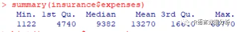
summarize the charges variable
summary(insurance$expenses)
histogram of insurance charges
hist(insurance$expenses)
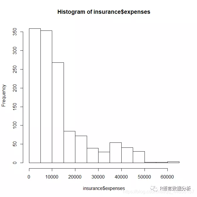
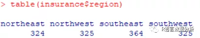
table of region
table(insurance$region)
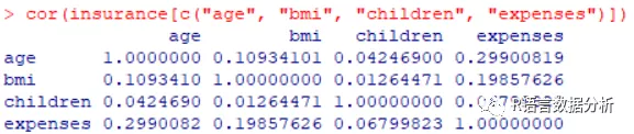
exploring relationships among features: correlation matrix
cor(insurance[c("age", "bmi", "children", "expenses")])
visualing relationships among features: scatterplot matrix
pairs(insurance[c("age", "bmi", "children", "expenses")])
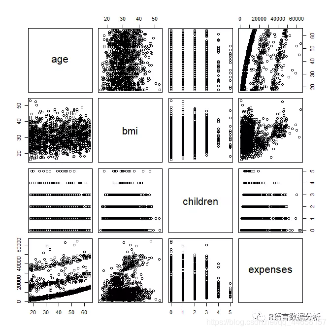
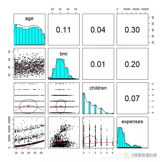
more informative scatterplot matrix
#install.packages('psych')
library(psych)
pairs.panels(insurance[c("age", "bmi", "children", "expenses")])
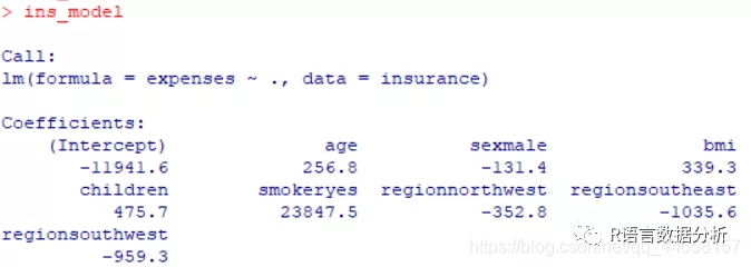
Step 2: Training a model on the data ----
ins_model <- lm(expenses ~ ., data = insurance)
see the estimated beta coefficients
ins_model
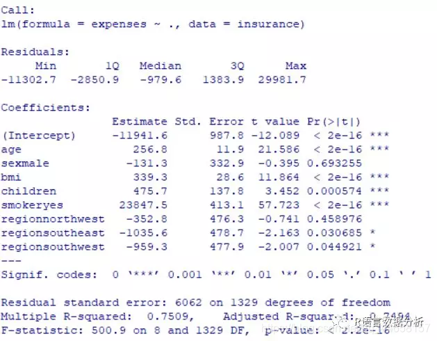
Step 3: Evaluating model performance ----
see more detail about the estimated beta coefficients
summary(ins_model)
Step 4: Improving model performance ----
add a higher-order “age” term
insurance$age2 <- insurance$age^2
add an indicator for BMI >= 30
insurance$bmi30 <- ifelse(insurance$bmi >= 30, 1, 0)
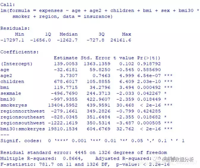
create final model
ins_model2 <- lm(expenses ~ age + age2 + children + bmi + sex +
                   bmi30*smoker + region, data = insurance)

summary(ins_model2)
Example: Estimating Wine Quality ----
Part 2: Regression Trees and Model Trees
Step 1: Exploring and preparing the data ----
wine <- read.csv("F:\\rwork\\Machine Learning with R (2nd Ed.)\\Chapter 06\\whitewines.csv")
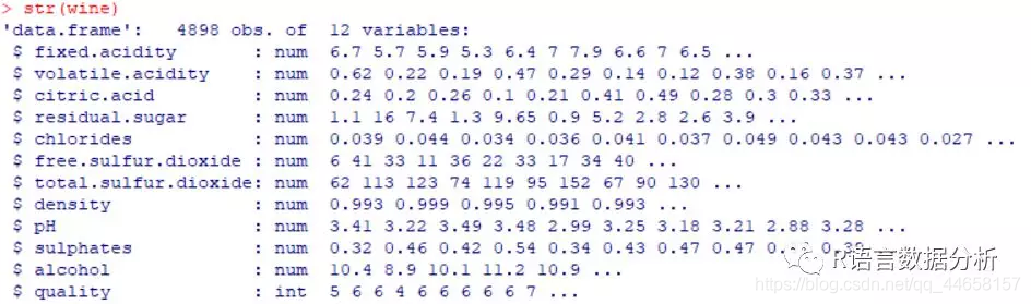
examine the wine data
str(wine)
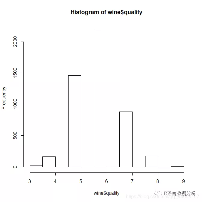
the distribution of quality ratings
hist(wine$quality)
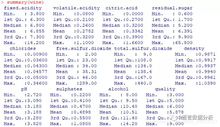
summary statistics of the wine data
summary(wine)
wine_train <- wine[1:3750, ]
wine_test <- wine[3751:4898, ]
Step 2: Training a model on the data ----
regression tree using rpart
library(rpart)
m.rpart <- rpart(quality ~ ., data = wine_train)
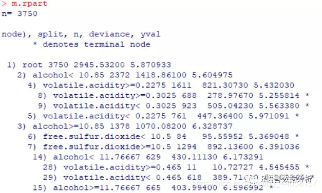
get basic information about the tree
m.rpart

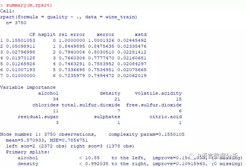
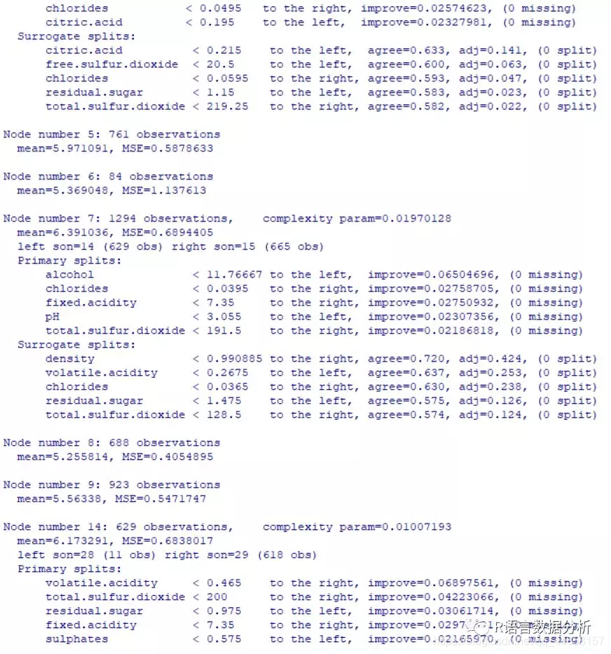
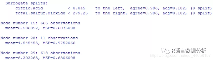
get more detailed information about the tree
summary(m.rpart)

use the rpart.plot package to create a visualization
#install.packages('rpart.plot')
library(rpart.plot)
a basic decision tree diagram
rpart.plot(m.rpart, digits = 3)
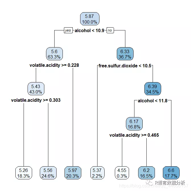
a few adjustments to the diagram
rpart.plot(m.rpart, digits = 4, fallen.leaves = TRUE, type = 3, extra = 101)

Step 3: Evaluate model performance ----
generate predictions for the testing dataset
p.rpart <- predict(m.rpart, wine_test)
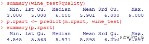
compare the distribution of predicted values vs. actual values
summary(p.rpart)
summary(wine_test$quality)
compare the correlation
cor(p.rpart, wine_test$quality)
function to calculate the mean absolute error
MAE <- function(actual, predicted) {
  mean(abs(actual - predicted))  }
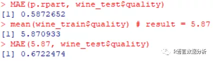
mean absolute error between predicted and actual values
MAE(p.rpart, wine_test$quality)
mean absolute error between actual values and mean value
mean(wine_train$quality) # result = 5.87
MAE(5.87, wine_test$quality)
Step 4: Improving model performance ----
train a M5’ Model Tree
library(RWeka)
m.m5p <- M5P(quality ~ ., data = wine_train)
display the tree
m.m5p
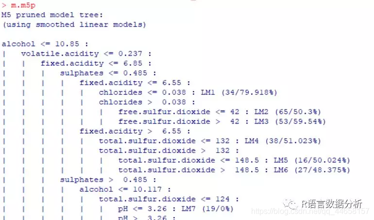
(信息过长,有163种情况,这里就不全部截图了)
get a summary of the model’s performance
summary(m.m5p)
generate predictions for the model
p.m5p <- predict(m.m5p, wine_test)
summary statistics about the predictions
summary(p.m5p)
correlation between the predicted and true values
cor(p.m5p, wine_test$quality)
mean absolute error of predicted and true values
(uses a custom function defined above)
MAE(wine_test$quality, p.m5p)
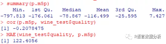
这里就得出了一个很奇怪的结论,因为一般来说使用先进的M5算法后模型的准确度会得到提高,即平均绝对误差(MAE)会减小,但是这次不减反增。大家可以自己选择数据试试,有问题留言哦~
