BP神经网络
1. 机器学习的三要素
1.1 模型
模型: 即待求解的参数。
模型简单来说就是使用什么映射函数来表示特征X和Y标签之间的关系F。
F有两种形式:F={f|y=f(x)} 或者 F={P|P(Y|X)}。
F={f|y=f(x)} 为决策函数,它表示的模型为非概率模型。F={P|P(Y|X)} 是条件概率表示,它的模型为概率模型。
1.2 策略
策略: 模型建立在参数上的评价指标。
通常我们使用损失函数来评价模型。
损失函数: 我们用损失函数度量错误的程度,也称之为代价函数。
通常损失函数值越小,模型就越好。
但训练时采用的损失函数不一定是评估时的损失函数。但通常二者是一致的。因为目标是需要预测未知数据的性能足够好,而不是对已知的训练数据拟合最好。
1.3 算法
算法: 即寻找模型中参数的迭代方向。
算法指学习模型的具体计算方法。通常采用数值计算的方法求解,如:批量梯度下降、随机梯度下降、随机批量梯度下降。
现通常使用随机批量梯度下降方法。
2. BP神经网络
BP神经网络的计算过程由正向计算过程和反向计算过程组成。
正向传播过程,输入模式从输入层经隐单元层逐层处理,并转向输出层,每一层神经元的状态只影响下一层神经元的状态。如果在输出层不能得到期望的输出,则转入反向传播,将误差信号沿原来的连接通路返回,通过修改各神经元的权值,使得误差信号最小。
2.1 训练过程流程图
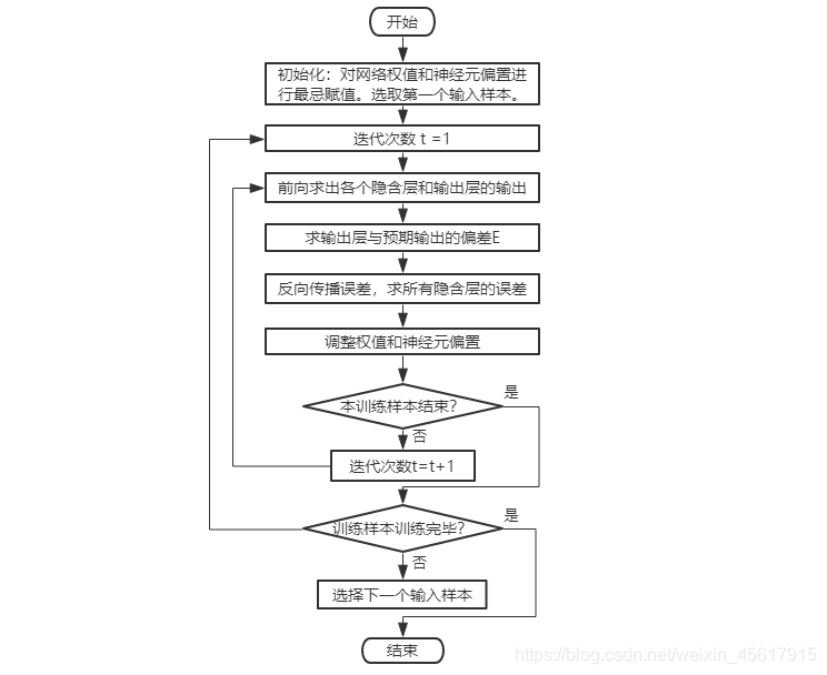
2.2 训练步骤
步骤1. 初始化网络权重
每两个 神经元之间的网络连接权重wij被初始化为一个很小的随机数,同时,每个神经元有一个偏置θi,也被初始化为一个随机数。
对每个样本x,按步骤二处理。
步骤2. 向前传播输入(前馈型网络)
根据训练样本x提供网络的输入层,通过计算得到每个神经元的输出。每个神经元的计算方法相同,都是由其输入的线性组合得到。
步骤3.反向误差传播
由步骤2一路向前,最终在输出层得到是技术处,可以通过与预期输出相比较的到的输出单元j的误差。
得到的误差需要从后向前传播,前面一层单元 j 的误差可以通过和它链接的后面一层的所有单元 k 的误差计算所得。
步骤4.网络权重与神经元偏置调整
在处理过程中,一边后向传播误差,一边调整网络权重和神经元的阈值。为方便起见,先计算得到所有神经元的误差,然后统一调整网络圈中和神经元的阈值。
调整权重的方法是从输入层与第一隐含层的连接权重开始,依次向后进行。
神经元偏置的调整方法是对每个神经元 j 进行如公式 θj=θj+△θ
+(η)Ej 所示的更新。
其中η是学习率,通常取0~1之间的常数。该参数也会影响算法的性能,太小的学习率会导致学习进行得慢,而太大的学习率可能回事算法出现不适当的解之间振动的情况。
经过查阅资料可得:将学习率设置为迭代次数 t 的倒数,即1/t。
步骤5.判断结束
对于每个样本,如果最终的输出误差小于可接受的范围或者迭代次数t达到了一定的阈值,则选取下一个样本,转到步骤2重新继续执行;否则,迭代次数t加1,然后转向步骤2继续使用当前样本进行训练。
3. 代码
3.1 BP神经网络的构建
代码:
% BP网络
% BP神经网络的构建
net=newff([-1 2;0 5],[3,1],{'tansig','purelin'},'traingd')
net.IW{1}
net.b{1}

p=[1;2];
a=sim(net,p)
net=init(net);
net.IW{1}
net.b{1}
a=sim(net,p)
%net.IW{1}*p+net.b{1}
p2=net.IW{1}*p+net.b{1}
a2=sign(p2)
a3=tansig(a2)
a4=purelin(a3)
net.b{2}
net.b{1}

net.IW{1}
net.IW{2}
0.7616+net.b{2}
a-net.b{2}
(a-net.b{2})/ 0.7616
help purelin

p1=[0;0];
a5=sim(net,p1)
net.b{2}
运行结果:
>> BP
net =
   Neural Network
              name: 'Custom Neural Network'
          userdata: (your custom info)

    dimensions:

         numInputs: 1
         numLayers: 2
        numOutputs: 1
    numInputDelays: 0
    numLayerDelays: 0
 numFeedbackDelays: 0
 numWeightElements: 13
        sampleTime: 1

    connections:

       biasConnect: [1; 1]
      inputConnect: [1; 0]
      layerConnect: [0 0; 1 0]
     outputConnect: [0 1]

    subobjects:

             input: Equivalent to inputs{1}
            output: Equivalent to outputs{2}

            inputs: {1x1 cell array of 1 input}
            layers: {2x1 cell array of 2 layers}
           outputs: {1x2 cell array of 1 output}
            biases: {2x1 cell array of 2 biases}
      inputWeights: {2x1 cell array of 1 weight}
      layerWeights: {2x2 cell array of 1 weight}

    functions:

          adaptFcn: 'adaptwb'
        adaptParam: (none)
          derivFcn: 'defaultderiv'
         divideFcn: (none)
       divideParam: (none)
        divideMode: 'sample'
           initFcn: 'initlay'
        performFcn: 'mse'
      performParam: .regularization, .normalization
          plotFcns: {'plotperform', plottrainstate,
                    plotregression}
        plotParams: {1x3 cell array of 3 params}
          trainFcn: 'traingd'
        trainParam: .showWindow, .showCommandLine, .show, .epochs,
                    .time, .goal, .min_grad, .max_fail, .lr

    weight and bias values:

                IW: {2x1 cell} containing 1 input weight matrix
                LW: {2x2 cell} containing 1 layer weight matrix
                 b: {2x1 cell} containing 2 bias vectors

    methods:

             adapt: Learn while in continuous use
         configure: Configure inputs & outputs
            gensim: Generate Simulink model
              init: Initialize weights & biases
           perform: Calculate performance
               sim: Evaluate network outputs given inputs
             train: Train network with examples
              view: View diagram
       unconfigure: Unconfigure inputs & outputs


ans =

    0.9793    0.7717
    1.5369    0.3008
   -1.0989   -0.7114


ans =

   -4.8438
   -1.5204
   -0.0970


a =

    0.5105


ans =

   -1.6151   -0.0414
    1.3628    0.5217
    1.2726   -0.5981


ans =

    3.3359
   -1.9858
    3.2839


a =

    1.6873


p2 =

    1.6380
    0.4205
    3.3602


a2 =

     1
     1
     1


a3 =

    0.7616
    0.7616
    0.7616


a4 =

    0.7616
    0.7616
    0.7616


ans =

    0.9190


ans =

    3.3359
   -1.9858
    3.2839


ans =

   -1.6151   -0.0414
    1.3628    0.5217
    1.2726   -0.5981


ans =

     []


ans =

    1.6806


ans =

    0.7683


ans =

    1.0088

a5 =

    0.5450


ans =

    0.9190

>>
代码说明:
newff()函数
该函数用于创建一个前馈BP神经网络。
句法:
net=netff(P,T,S,TF,BTF,BLF,PF,IPF,OPF,DDF)
P:输入数据矩阵
T:目标数据矩阵
S:隐含层节点数
TF:节点传递函数(阈值函数hardlim,hardlims,线性函数purelin,双曲正切S型函数tansig,对数S型传递函数)
BTF:训练函数(梯度下降训练函数traingd,动量反传梯度下降函数traingdm,动态自适应学习率下降函数traingda,动量反传和动态自适应梯度下降训练函数traindx,L_M训练函数trainlm)
BLF:网络学习函数,(BP学习规则learngd,带动量的BP学习规则learngdm)
PF:性能分析函数(均值绝对误差性能分析函数mae,均方差性能分析函数mse)
IPF:输入处理函数
OPF:输出处理函数
DDF:验证数据划分函数
init()函数重新将整个网络的权值和阈值初始化,将权值和阈值重新归零。
代码:
% BP网络
% BP神经网络的构建
net=newff([-1 2;0 5],[3,1],{'tansig','purelin'},'traingd')
net.IW{1}
net.b{1}
%p=[1;];
p=[1;2];
a=sim(net,p)
net=init(net);
net.IW{1}
net.b{1}
a=sim(net,p)
net.IW{1}*p+net.b{1}
p2=net.IW{1}*p+net.b{1}
a2=sign(p2)
a3=tansig(a2)
a4=purelin(a3)
net.b{2}
net.b{1}

P=[1.2;3;0.5;1.6]
W=[0.3 0.6 0.1 0.8]
net1=newp([0 2;0 2;0 2;0 2],1,'purelin');
net2=newp([0 2;0 2;0 2;0 2],1,'logsig');
net3=newp([0 2;0 2;0 2;0 2],1,'tansig');
net4=newp([0 2;0 2;0 2;0 2],1,'hardlim');

net1.IW{1}
net2.IW{1}
net3.IW{1}
net4.IW{1}
net1.b{1}
net2.b{1}
net3.b{1}
net4.b{1}


net1.IW{1}=W;
net2.IW{1}=W;
net3.IW{1}=W;
net4.IW{1}=W;

a1=sim(net1,P)
a2=sim(net2,P)
a3=sim(net3,P)
a4=sim(net4,P)

init(net1);
net1.b{1}

help tansig
运行结果:
>> BP
net =
   Neural Network

              name: 'Custom Neural Network'
          userdata: (your custom info)

    dimensions:

         numInputs: 1
         numLayers: 2
        numOutputs: 1
    numInputDelays: 0
    numLayerDelays: 0
 numFeedbackDelays: 0
 numWeightElements: 13
        sampleTime: 1

    connections:

       biasConnect: [1; 1]
      inputConnect: [1; 0]
      layerConnect: [0 0; 1 0]
     outputConnect: [0 1]

    subobjects:

             input: Equivalent to inputs{1}
            output: Equivalent to outputs{2}

            inputs: {1x1 cell array of 1 input}
            layers: {2x1 cell array of 2 layers}
           outputs: {1x2 cell array of 1 output}
            biases: {2x1 cell array of 2 biases}
      inputWeights: {2x1 cell array of 1 weight}
      layerWeights: {2x2 cell array of 1 weight}

    functions:

          adaptFcn: 'adaptwb'
        adaptParam: (none)
          derivFcn: 'defaultderiv'
         divideFcn: (none)
       divideParam: (none)
        divideMode: 'sample'
           initFcn: 'initlay'
        performFcn: 'mse'
      performParam: .regularization, .normalization
          plotFcns: {'plotperform', plottrainstate,
                    plotregression}
        plotParams: {1x3 cell array of 3 params}
          trainFcn: 'traingd'
        trainParam: .showWindow, .showCommandLine, .show, .epochs,
                    .time, .goal, .min_grad, .max_fail, .lr

    weight and bias values:

                IW: {2x1 cell} containing 1 input weight matrix
                LW: {2x2 cell} containing 1 layer weight matrix
                 b: {2x1 cell} containing 2 bias vectors

    methods:

             adapt: Learn while in continuous use
         configure: Configure inputs & outputs
            gensim: Generate Simulink model
              init: Initialize weights & biases
           perform: Calculate performance
               sim: Evaluate network outputs given inputs
             train: Train network with examples
              view: View diagram
       unconfigure: Unconfigure inputs & outputs


ans =

   -0.3285    0.9497
   -0.5719   -0.9072
    1.6154   -0.0374


ans =

    0.2148
    2.5540
    1.7106


a =

    0.8726


ans =

   -0.8941   -0.8081
    0.6896   -0.8773
    1.6165   -0.0102


ans =

    4.8922
    1.8484
    1.6422


a =

    0.3126


ans =

    2.3819
    0.7834
    3.2382


p2 =

    2.3819
    0.7834
    3.2382


a2 =

     1
     1
     1


a3 =

    0.7616
    0.7616
    0.7616


a4 =

    0.7616
    0.7616
    0.7616


ans =

   -0.5524


ans =

    4.8922
    1.8484
    1.6422


P =

    1.2000
    3.0000
    0.5000
    1.6000


W =

    0.3000    0.6000    0.1000    0.8000


ans =

     0     0     0     0


ans =

     0     0     0     0


ans =

     0     0     0     0


ans =

     0     0     0     0


ans =

     0


ans =

     0


ans =

     0


ans =

     0


a1 =

    3.4900


a2 =

    0.9704


a3 =

    0.9981


a4 =

     1


ans =

     0

>>
代码及运行结果说明:
sign(x):符号函数 (Signum function)。
当x<0时,sign(x)=-1;
当x=0时,sign(x)=0;
当x>0时,sign(x)=1。
tansig(x)= 2/(1+exp(-2*x))-1,是sigmoid函数。
purelin(x):线性传递函数。
3.2 BP神经网络的训练
代码:
p=[-0.1 0.5]
t=[-0.3 0.4]
w_range=-2:0.4:2;
b_range=-2:0.4:2;
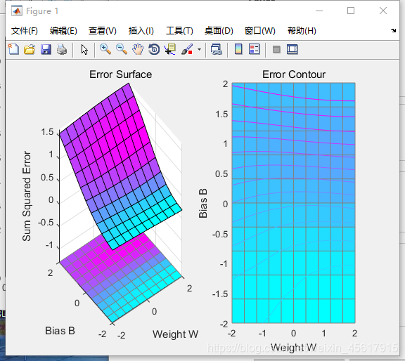
ES=errsurf(p,t,w_range,b_range,'logsig');%单输入神经元的误差曲面
plotes(w_range,b_range,ES)%绘制单输入神经元的误差曲面
pause(0.5);
hold off;
net=newp([-2,2],1,'logsig');
net.trainparam.epochs=100;
net.trainparam.goal=0.001;
figure(2);
[net,tr]=train(net,p,t);
title('动态逼近')
wight=net.iw{1}
bias=net.b
pause;
close;
运行结果:
>> BP

p =

   -0.1000    0.5000


t =

   -0.3000    0.4000


wight =

   15.1653


bias =

    [-8.8694]
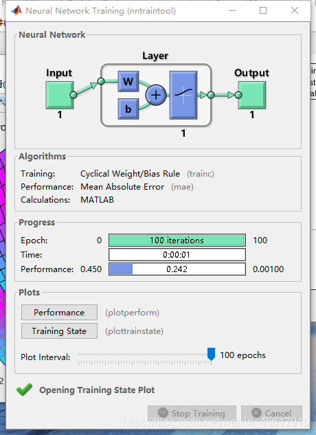
nntraintool窗口:
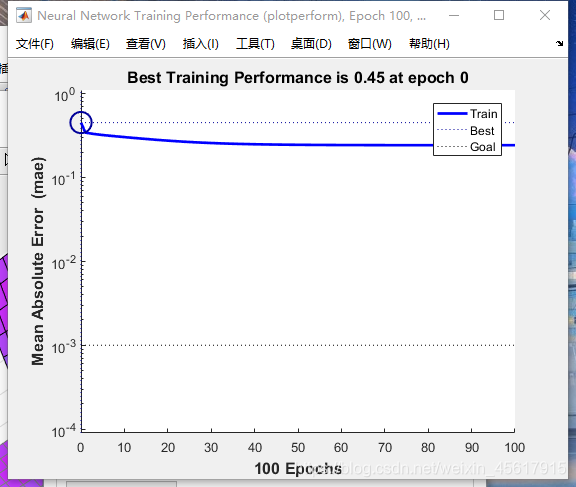
Performance绘图结果:
代码及运行结果说明:
ES=errsurf(p,t,w_range,b_range,‘logsig’):
单输入神经元的误差曲面。
plotes(w_range,b_range,ES):
绘制单输入神经元的误差曲面。
net.trainParam.epochs:
定义神经网络net的循环次数。
net.trainparam.goal:
设置训练目标最小误差值。
train()函数:用于训练一个神经网络。
网络训练函数是一个通用的学习函数,训练函数重复的把一组输入向量应用到一个网络上,每次都更新网络,直到达到某种准则。停止准则的可能是最大的学习次数,最小的误差梯度或者误差目标。
[net,tr,y,e,pf,af]=train(net,p,t,pi,ai)
[net,tr,y,e,pf,af]中,net 是训练后的网络,tr为训练纪录,y为网络输出,e为误差向量;pf为训练终止时的输入延时状态,af为训练终止时的层延时状态;
train(net,p,t,pi,ai)中,net为训练之前的网络,p为网络的输入向量矩阵;t表示网络的目标矩阵,默认值是0;pi表示初始输入延时,默认值是0;ai表示初始的层延时,默认值是0;
代码:
% 练
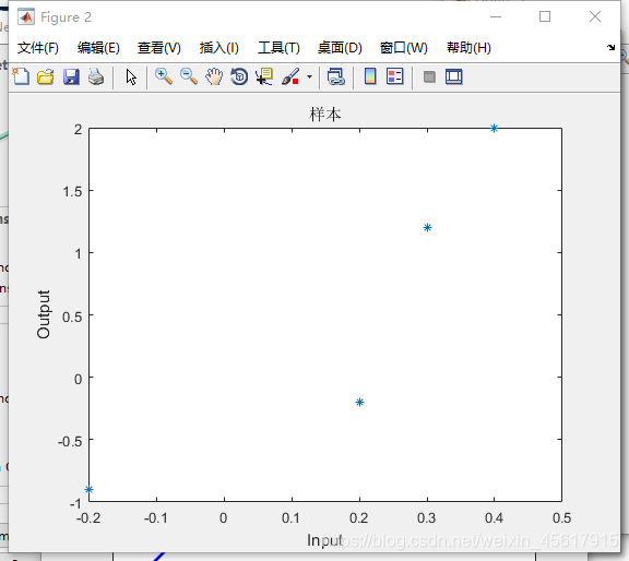
p=[-0.2 0.2 0.3 0.4]
t=[-0.9 -0.2 1.2 2.0]
h1=figure(1);
net=newff([-2,2],[5,1],{'tansig','purelin'},'trainlm');
net.trainparam.epochs=100;
net.trainparam.goal=0.0001;
net=train(net,p,t);
a1=sim(net,p)
pause;
h2=figure(2);
plot(p,t,'*');
title('样本')
title('样本');
xlabel('Input');
ylabel('Output');
pause;
hold on;
ptest1=[0.2 0.1]
ptest2=[0.2 0.1 0.9]
a1=sim(net,ptest1);
a2=sim(net,ptest2);
net.iw{1}
net.iw{2}
net.b{1}
net.b{2}
运行结果:
>> BP

p =

   -0.2000    0.2000    0.3000    0.4000


t =

   -0.9000   -0.2000    1.2000    2.0000


a1 =

   -0.9000   -0.1999    1.1999    2.0000


ptest1 =

    0.2000    0.1000


ptest2 =

    0.2000    0.1000    0.9000


ans =

    3.4994
    9.9514
    3.7383
    3.4868
    3.5000


ans =

     []


ans =

   -7.0014
   -2.6098
    3.3197
    3.4796
    7.0000


ans =

   -0.1984

>>
nntraintool窗口:

样本绘图结果:
Performance绘图结果:

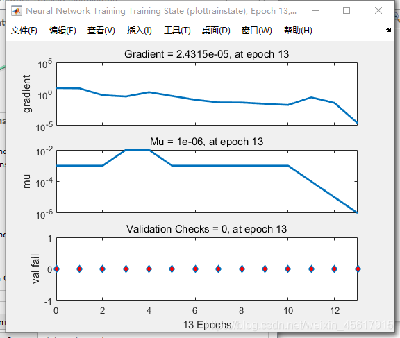
Training Stata绘图结果:
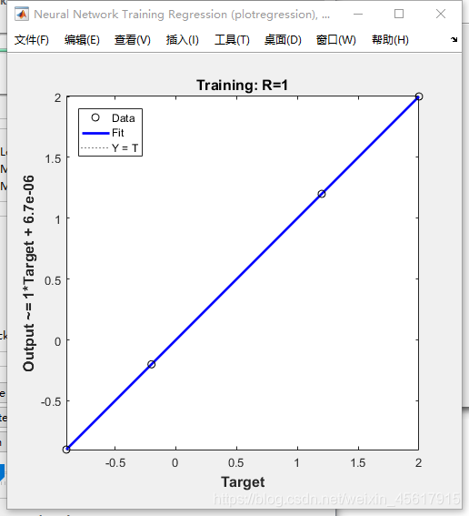
Regression绘图结果:
代码及运行结果说明:
Neural Network Training(nntraintool)界面
1.Neural Network
这里显示的是输入大小,中间层数量以及每层的神经元个数。
2.Algorithms
Training:Levenberg-Marquardt。这表示学习训练函数。
Performance:Mean Squared Error。这表示性能用均方误差来表示。
Calculations: MEX。
3.Progress
Epoch:迭代次数。
Time:运行时间。
Performance:训练数据集的性能。
Gradient:梯度。
Mu:变量mu确定了学习是根据牛顿法还是梯度法来完成,下式为更新参数的L-M规则:
% jj = jX * jX
% je = jX * E
% dX = -(jj+I*mu) \ je
随着mu的增大,LM的项jj可以忽略。因此学习过程主要根据梯度下降即mu/je项,只要迭代使误差增加,mu也就会增加,直到误差不再增加为止,但是,如果mu太大,则会使学习停止,当已经找到最小误差时,就会出现这种情况,这就是为什么当mu达到最大值时要停止学习的原因。
Validation Checks:最大验证失败次数。
(解释:比如默认是6,则系统判断这个验证集误差是否在连续6次检验后不下降,如果不下降或者甚至上升,说明training set训练的误差已经不再减小,没有更好的效果了,这时再训练就没必要了,就停止训练,不然可能陷入过拟合。)
4.Plots (3个都可以点进去,会有相应的图出来)
Performance:通过均方差开衡量网络的性能,可以看出,迭代次数越多,性能越好。
Training tate:记录Gradient和Validation Checks,训练状态的跟踪.
Regression:通过绘制回归线来测量神经网络对应数据的拟合程度。
